Background
To introduce you to some of the fundamental ideas behind machine learning, we’ll start off with a lesson on perhaps the simplest type of supervised learning: linear regression. In it, you’ll learn what it means to create a machine learning model, and how we can evaluate and eventually train such models.
This chapter will be pretty math-heavy, so take your time getting through it if you have to. Almost everything we see from here will build on these ideas.
Many of the images in this lesson come from Andrew Ng’s Machine Learning course on Coursera. If you have time, we recommend that you give some of his videos a watch.
Introduction: The Regression Problem
In our first (introductory) lesson, we learned that supervised learning is a way to use labeled examples to teach a program to map from A (input) to B (output) — or in more mathematical terms, from x (input) to y (output). Regression is a specific type of supervised learning where both the input and output are continuous (e.g. numerical values, such as someone’s height), as opposed to discrete (e.g. classifying cats vs. dogs).
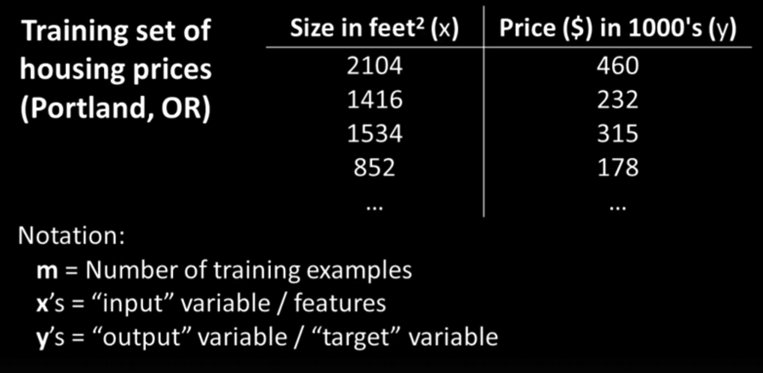
As an example, let’s imagine that we want to be able to predict the price of a house (y) from the size of the house (x), as measured in square feet. To help us do so, we have been giving a dataset of houses from Portland, Oregon. Each data point (or training example) includes information on the size of the house (our known input, AKA feature) and the house’s price (what we want to eventually be able to predict).
Let’s say that the dataset looks something like this:
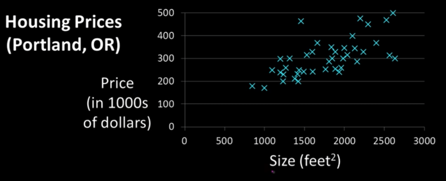
Our goal, then, is to use this dataset (or training set) to learn how to make a good guess about the price of any house given the house’s size. If you’ve taken a statistics course at any point, you may already have an idea of how to do so. We can plot each house as a datapoint on a graph, and then create a line of best fit that will allow us to determine how the size of a house affects its price, on average. So, you go ahead and place each house on a graph, and get something like this:
Our next step is to create a model from the current data so that we can use it for future prediction. Judging by the graph, it looks like a straight line may fit the data relatively well. Thus, we can create our model in terms of a linear function, which, in previous math classes, you may have seen written in the form: \(y = mx + b\).
This equation is all well and good, but in machine learning, we typically write out our linear regression models in a different form:
\[h_w(x) = w_0 + w_1x\]In this case, \(h_w(x)\) represents our hypothesis (also called a prediction), or our (educated) guess regarding the price of the house. The terms \(w_0\) and \(w_1\) are called the parameters of our model: as \(w_0\)(the y-intercept) and \(w_1\)(the slope) change, so does the shape of the line, and as a result, so does the model itself.
Once we pick some values for \(w_0\) and \(w_1\), we’ll be able to formulate our hypothesis as a simple function of x (the input, which in our case, is the size of the house). All we’d need to do to predict the price of a house is to find out how large the house is in square feet, and then feed that measurement as our \(x\) value into the model.
(Note: The lone \(w_0\) term is sometimes referred to as a “bias,” and thus denoted with a \(b\) instead, but for now we’ll just keep it as \(w_0\). The \(w_1\) term can also be called a “weight,” since it describes how much we want to weigh our knowledge of the size of the house into our final price prediction. This terminology will make a bit more sense once we get to problems with more than one feature.
In some instances, such as in Andrew Ng’s machine learning course, \(\theta\) may be used instead of \(w\). Both symbols refer to the parameters of the model, so they’re more or less interchangeable. However, when we get to neural networks, we’ll see that most people use \(w\) to refer to the weights of a model, so we’ll go ahead and follow that convention from the start.)
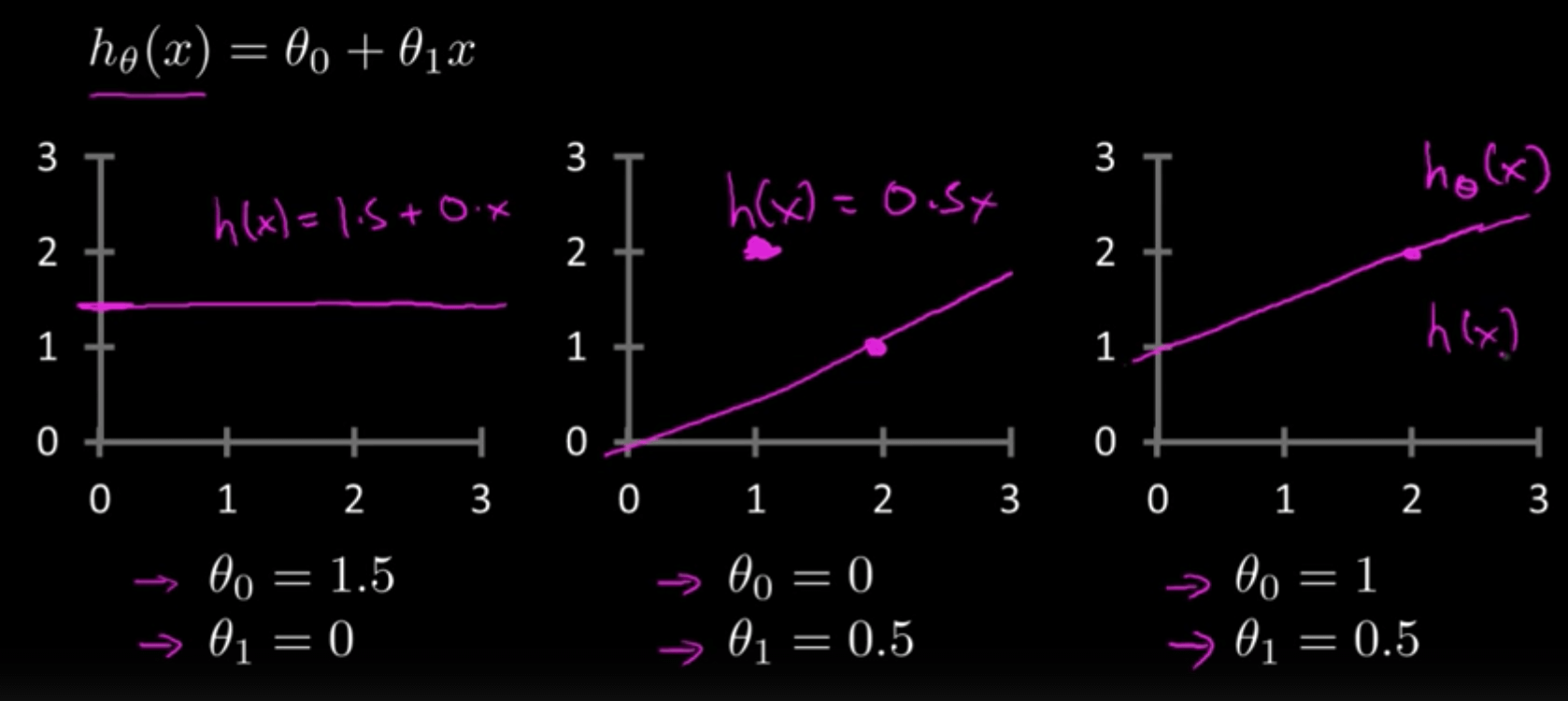
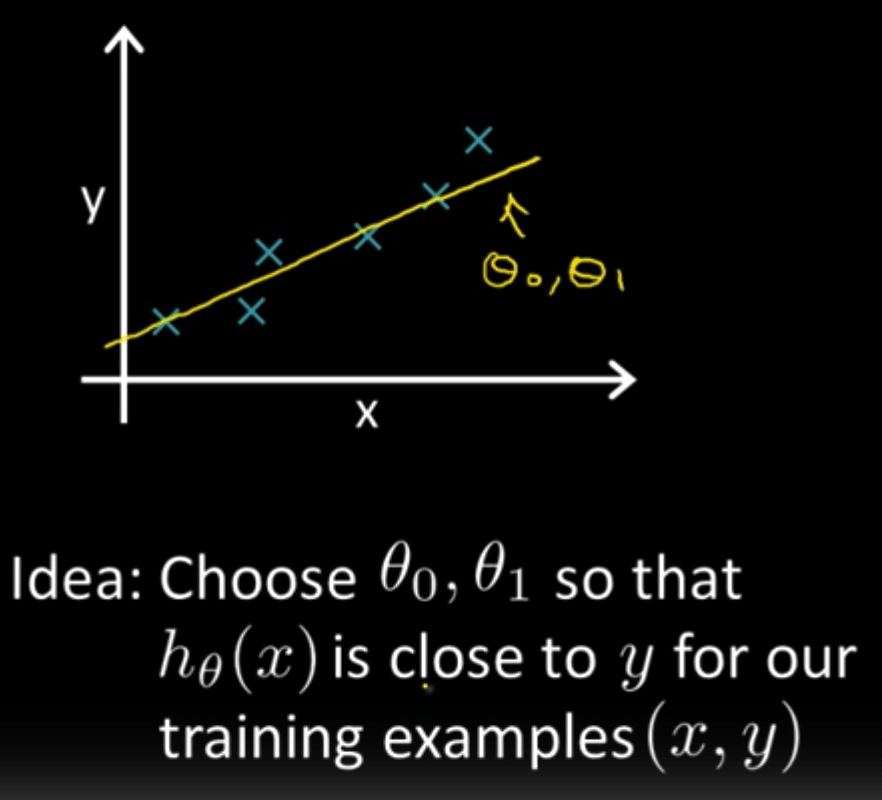
As you can see, we will get different shapes depending on the values that we pick for the parameters of our network (\(w_0\) and \(w_1\)). Our goal, then, should be to pick values for our parameters so that our model (or our regression line) fits our training data well. If we can find a good set of values for \(w_0\) and \(w_1\), then we should be able to make accurate predictions about the price of any house, even if the house isn’t in our existing dataset.
In order to decide exactly what values to use for our parameters, though, we’ll need to define what exactly it means for a model (and its parameters) to be “good” — an idea that we’ll explore in the following section.
Evaluation: Cost Functions
Before being able to find the optimal model to fit our training data, we’ll first need a way to numerically describe how good our model is. To do so, we’ll introduce what’s called a cost function: a measurement of the error of our model with respect to the actual data that we have. Once we have this error measurement, we’ll be able to pick parameter values that minimize the cost function, thereby giving us the most optimal model.
As we’ll see later, there are plenty of different cost functions out there. In this lesson though, we’ll focus one of the most widely used cost functions (especially for regression problems): the “mean squared error” (MSE). For each of the \(i\) data points in our training set of size \(m\), we’ll look at what our model would hypothesize the output to be given the input \((h_w(x^{(i)})\), where \(x\) is the size of the house), versus the actual output (e.g. the actual price, \(y(i)\)), and calculate the error between the two. As the name suggests, we’ll then square the error to give an extra large penalty to very erroneous predictions, and then average these squared-errors over all training examples. (As a last step, we’ll divide the whole thing by two to make the math easier later on.)
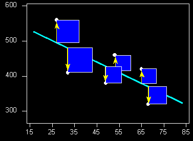
In the above diagram, each box represents the squared-error for one data point. Our objective, then, should be to minimize the total (or average) size of those boxes. To do this, we’ll need to write out our MSE cost function (typically denoted with the function \(J\) in mathematical terms:
\[MSE \;Cost = J(w_0, w_1) = {\frac1{2m}}\sum_{i=0}^m(h_w(x^{(i)})-y^{(i)})^2\]Take a while to just look at this function definition if you have to. Starting with the right side of the equation: the \(i\) superscripts denote different training examples, while the \(m\) refers to the total number of training examples in our data set. Working our way from the inside out, we can see that we take the difference (or error) between our predicted price \(h_w(x^{(i)})\) and the actual price \(y^{(i)}\) for a certain training example, square this error, and then average over all training examples by summing the errors up and dividing by the number of examples (\(m\)). (We throw in a 2 in the denominator to make the math easier in the optimization step, where we’ll have to differentiate the cost function to find its minimum, allowing the 2 in the exponent to cancel out with the 2 in the denominator.)
If we want, we can substitute in our definition of \(h_w(x)\) into the cost function, making it more clear how \(J\) is a function of our parameters \(w_0\) and \(w_1\). (You can think of \(x\) and \(y\) as constants, since they represent fixed data points in our training set.)
\[J(w_0, w_1) = {\frac1{2m}}\sum_{i=0}^m((w_0 + w_1x^{(i)}) - y^{(i)})^2\]What this equation means is that as we change the parameters of our model, we directly change the shape of our regression line, affecting how large our error terms (and subsequently, the cost) will be. In fact, just like how we would plot any other function, we can try out some different values for \(w_0\) and \(w_1\), observe the cost that we get, and plot the results on a 3D graph.
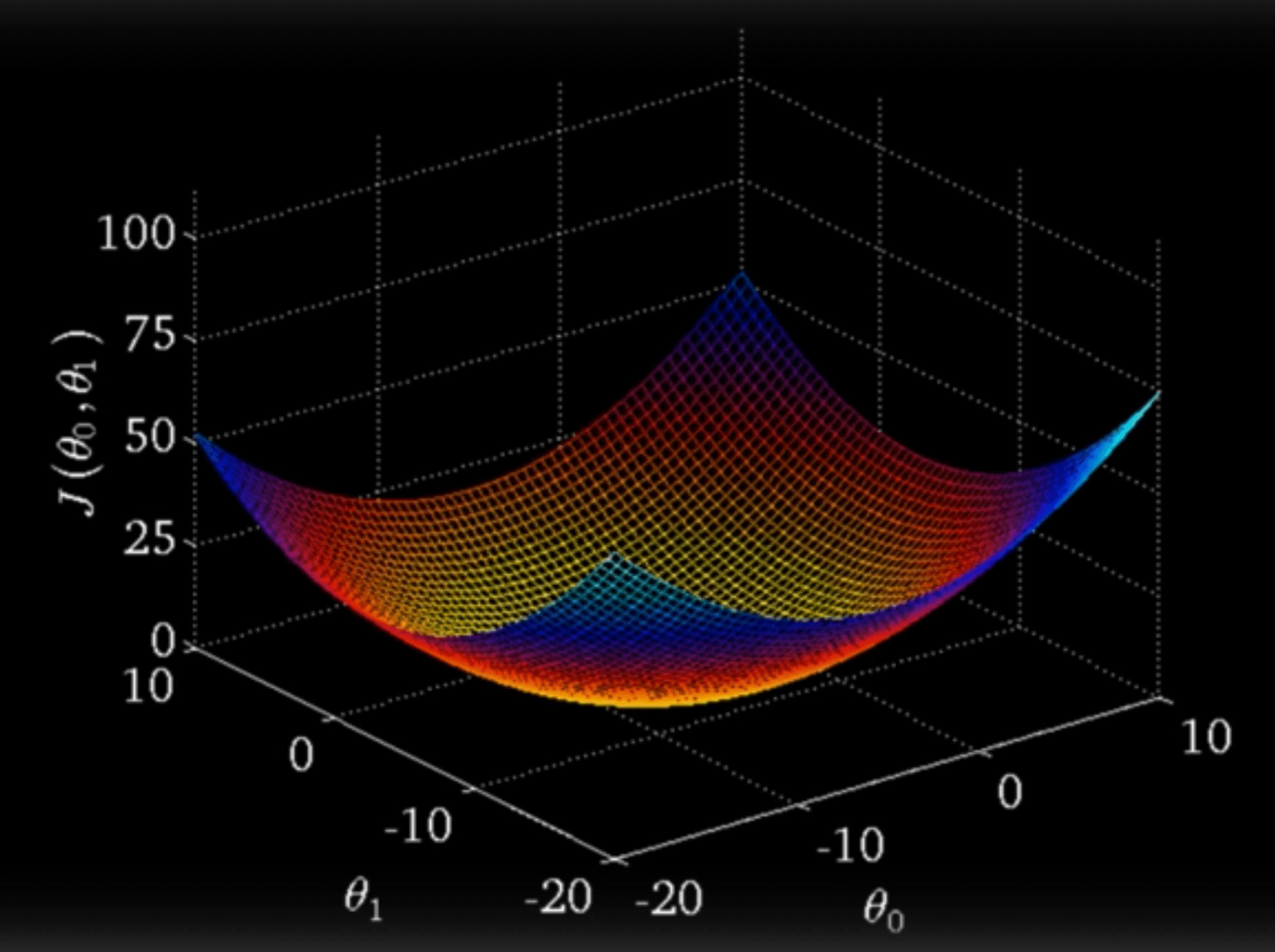
Notice that the curve we get is convex, or bowl-shaped, meaning that there is only one minimum point. While not every cost function will have a convex graph, the fact that this specific graph is convex allows for some convenient properties. At the bottom of the curve, we have a set of parameters that provides the best fit for the training data, resulting in the minimum possible cost for our model. As we stray from these ideal parameter values, the regression line gets shifted further away from our actual data, resulting in an increase in the cost. Since our graph is completely convex, it is guaranteed that our minimum is a global minimum, as opposed to just a local one.
Our next step, then, should be to find out how exactly to discover the best possible values for \(w_0\) and \(w_1\) so that we end up at this minimum point. To do so, we’ll introduce a learning algorithm that is at the very core of modern machine learning/deep learning: gradient descent.
\(\text{Objective: find optimal } w_0,w_1 \text{ that minimize }J(w_0,w_1)\)
Optimization: Gradient Descent
If you’ve taken a decent amount of calculus, then you may already have an idea of how we could potentially find the minimum point of the cost function: by finding where the partial derivatives of the cost, with respect to both \(w_0\) and \(w_1\) is equal to zero. (If you haven’t taken multivariate calculus yet, the partial derivative is still pretty easy to understand: it’s the derivative of a function with respect to one of its inputs, if you hold the other inputs constant.)
While this analytical solution may seem appealing at first, it tends to be far too computationally expensive for more complex problems (i.e. problems with many more inputs/features). In these cases, gradient descent usually turns out to be a much more effective solution.
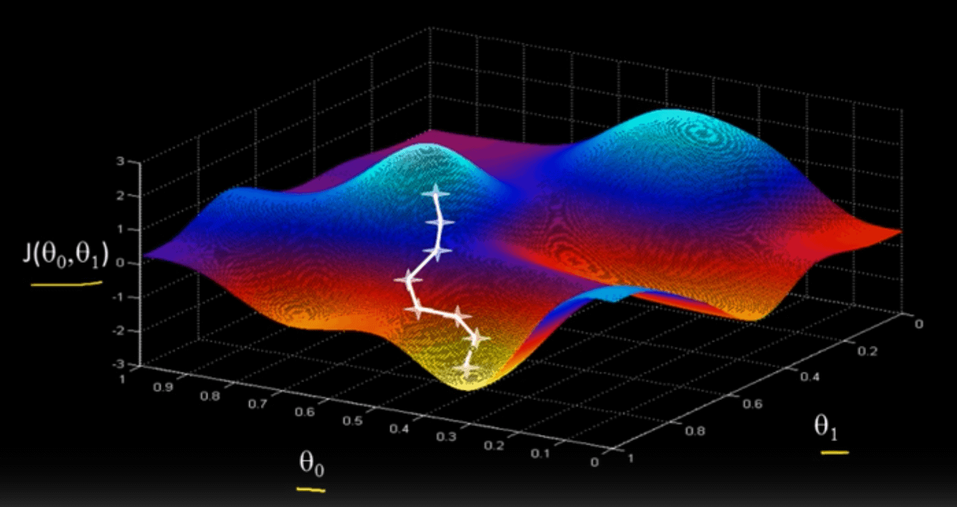
Before we get more into the math behind gradient descent, here’s a brief analogy that illustrates how it works: Let’s imagine that you’re stuck somewhere with lots of hilly terrain, and for whatever reason, you want to find your way to the bottom of a valley. Normally, you’d just take a look around to see where the deepest valley is, but since there’s a dense fog all around you, you can only look a few feet in any direction. Given these constraints, you make a plan of action: you first look around you to see which direction slants downward, and you take a small step in that direction, causing you to end up at a new point. From there, you then look around again, and take a step in the downward direction. You repeat this process until eventually, you find yourself at a minimum point, from which you can’t seem to go any lower. At last, you decide to stop at this point and take a well-deserved rest.
We can imagine our optimization problem, in which we want to find the minimum point of our cost function, in a similar way. (Remember that the cost is a function of our parameters, meaning that we want to find the values of our parameters such that we end up with the lowest possible cost.) We can imagine \(w_0\) and \(w_1\) as our \(x\) and \(y\) coordinates, and the cost \(J\) as our elevation. Since we initially don’t know where the minimum is, we decide to start off with some small random values for both \(w_0\) and \(w_1\), placing us on a random point on the cost function graph. From this point, we want to find out which direction is “down” — in other words, what small changes in \(w0\) and \(w1\) will cause the cost to decrease.
To do this, we’ll calculate the gradient of the cost function, or the slope of the cost function in each direction. In more mathematical terms, the gradient is the partial derivative of the output (the cost) with respect to each of the inputs (our parameters). Knowing the gradient allows us the answer the question: if I shift \(w_0\) and \(w_1\) by just a tiny bit, how will the cost change? Once we have this gradient, we’ll be able to change \(w_0\) and \(w_1\) by a small amount so that we descend down our cost function graph, placing us at a slightly lower point on the graph. We then re-calculate the gradient at this new point, and take another step in the “down” direction. We repeat this process until we eventually converge at a local (or hopefully, global) minimum, where the parameter values result in a model with the best possible fit for our training data.
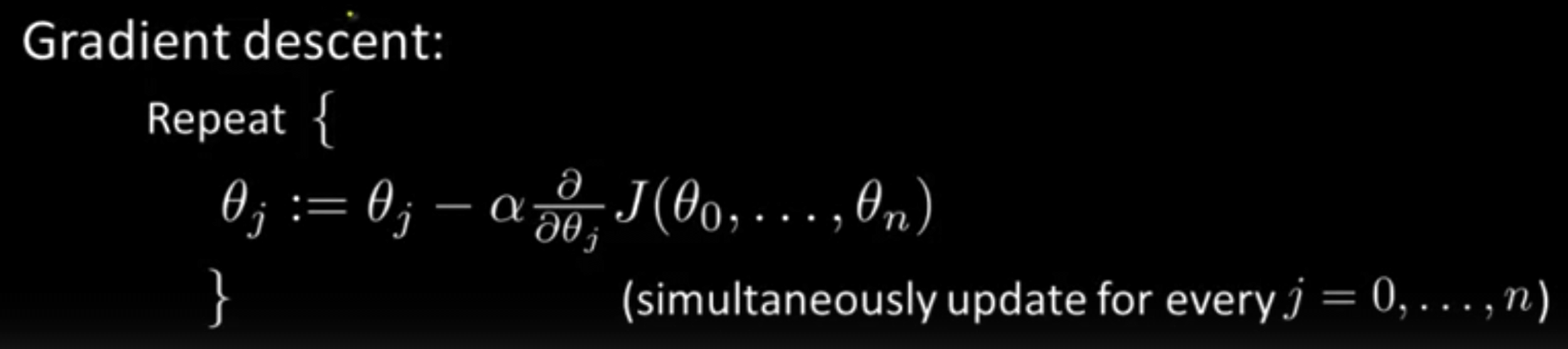
In mathematical terms, the gradient descent algorithm can be formally written out as:
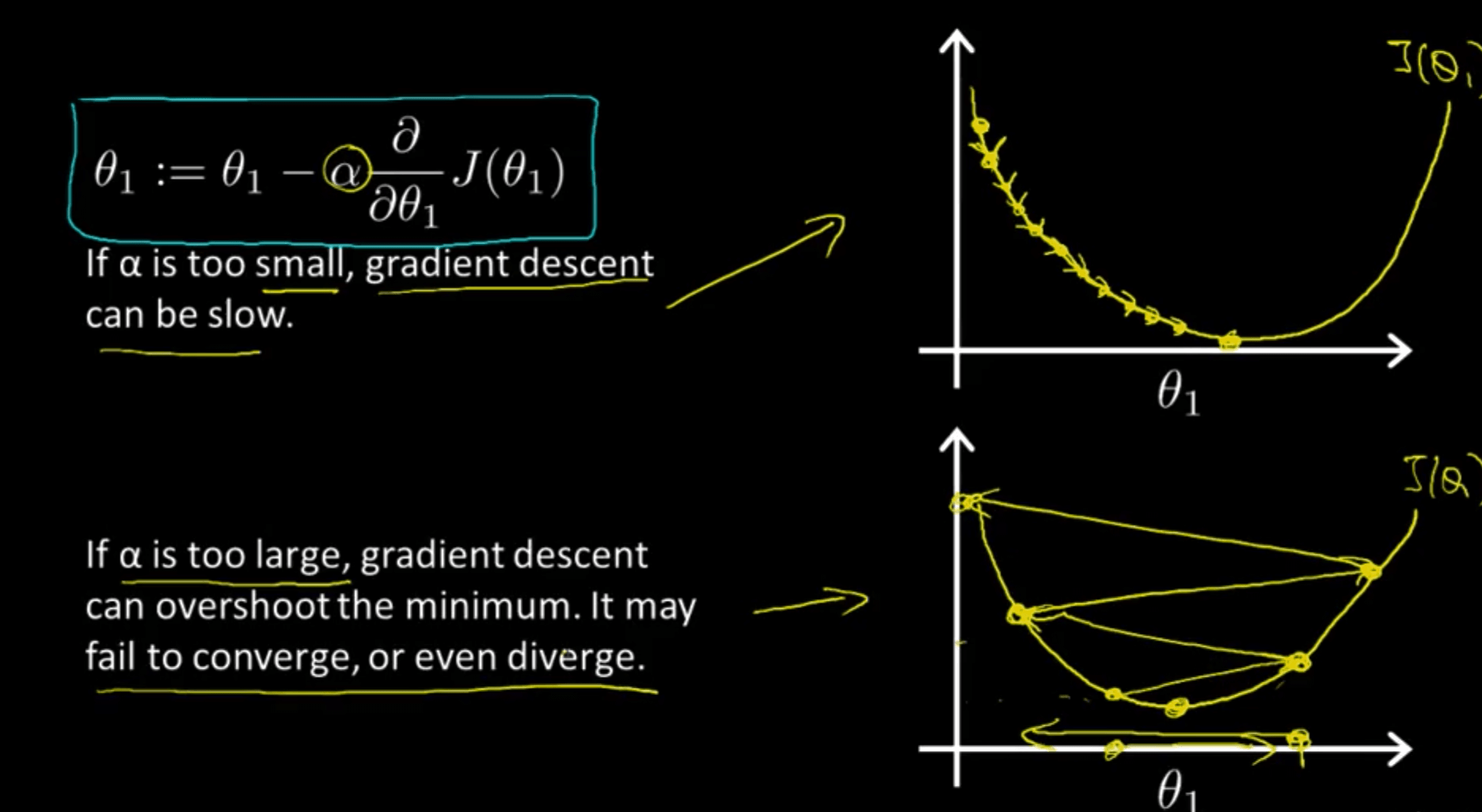
\[\text{Repeat Until Convergence:}\qquad w_j:=w_j−\alpha\frac{\partial (J(w_0,w_1))}{\partial w_j}\qquad \forall j \in \{0,1\}\]This may seem a bit intimidating at first, but it’s a worthwhile exercise to try to parse it out. On the very right, you can see that we first take the partial derivative of the cost function with respect to each parameter \(w_j\). This tells us how the cost will change if we decide to shift \(w_j\) a tiny bit in the positive direction. We then scale this value by some amount \(\alpha\) (which we’ll discuss in a moment), and then use it to update \(w_j\) accordingly. We use subtraction in our update because we want to move in the downward direction of our cost function graph. By repeatedly updating each of our parameters in this way, we gradually move our line of best fit closer and closer to the training data, until we end up with our final model.
We define \(\alpha\) as the learning rate, which determines how large each downward step will be. Choosing a good learning rate can be an art in itself: too small and our model will learn too slowly; too large and we may end up overshooting the minimum once we get to the bottom, causing our gradient descent algorithm to diverge (i.e. bounce back and forth) rather than converge at the actual minimum.
For our linear regression problem, the partial derivative terms are relatively easy to evaluate. Once we apply the power rule and chain rule to differentiate the cost function with respect to \(w_0\) and \(w_1\), we get these equations as our gradient descent updates:
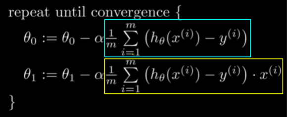
The red box contains the evaluated expression for \(\frac{\delta }{\delta w_{0}}J\), and the blue box contains the evaluated expression for \(\frac{\delta }{\delta w_{1}}J\) If you don’t completely understand these equations at first, that’s fine — what’s more important for now is that you understand the intuition behind cost functions and how we can optimize our model parameters by using gradient descent. If you would like more of a step-by-step demonstration of how we arrive at these equations, we recommend watching the videos below:
While gradient descent is great for minimizing our cost, a lower cost doesn’t always make for a better model. For example, we can add polynomial terms to our model (i.e. line of best fit) if we want, but we have to be careful when doing so. Take a look at the graphic below: while the more complex model on the right has a very low cost, since the curve essentially passes through each of the data points, it wouldn’t do a good job of generalizing to new data — in other words, the model model is overfit to the training data.
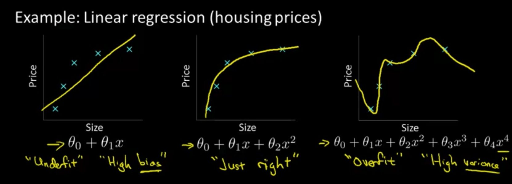
Remember that our original motivation for creating a model was so that we could make predictions for some output given some input(s). Our training examples were there to help us learn to make these predictions, but they weren’t the focus of our machine learning problem itself. In other words, we wanted to generalize beyond just the training data so that our model would work for new examples as well. As demonstrated above, a simpler model can sometimes be better at accomplishing this than a needlessly complex one.
Extension: Linear Regression with Multiple Variables
While the above methods work great for solving machine learning problems with only one input (e.g. the size of a house), almost every machine learning problem in real life has far more than just one input. Let’s say that now, instead of generating our prediction for the price of the house based on information about the house’s size alone, we want to factor in other features, such as the number of bedrooms it has, the age of the house, etc. To do so, we expand our training data to include more information about each house:
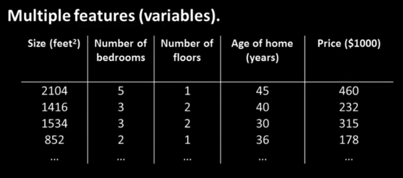
In order to account for all these features, we’re going to need a different way to define our hypothesis: instead of just scaling our one feature by \(w_1\) and adding on \(w_0\), we’ll “weight” each feature by a certain amount depending on how important we think it is to the final output, and then sum up all these terms to generate our prediction. For each feature \(x_1, x_2, …, x_n\), we’ll have a corresponding parameter \(w_1, w_2, ..., w_n\) that will act as our weight. (For example, if we think that the number of bedrooms that the house has is more important to the price than the number of floors, then the weight corresponding to the number of bedrooms will be larger than the weight corresponding to the number of floors.) We’ll keep the lone \(w_0\) term as well, so that we can shift the whole prediction up or down if doing so fits the data better.
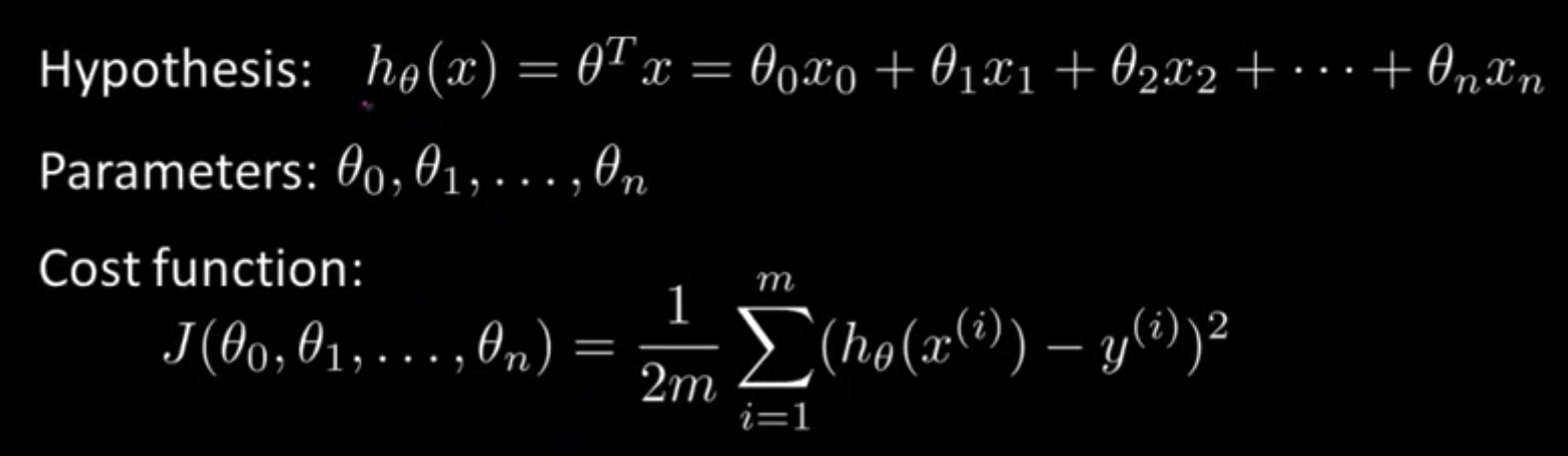
\[h_{w}(x) = w_0 + w_1x_1 + w_2x_2 + ... + w_nx_n\]If you’ve taken linear algebra, then you may recognize this type of weighted sum as a linear combination of our input features, which is a pretty good way to think about our new hypothesis formulation. If you’re familiar with matrices, you can also think of this weighted sum as a matrix multiplication of our feature vector (denoted with just \(x\)), which contains all our \(x_n\) input terms, and our parameter vector (denoted with either \(w\) or \(\theta\) ), which contains all our \(w_n\) (weight/parameter) terms. When we multiply the two vectors together, we get essentially the same equation as the one above, with each term listed out individually. If that doesn’t quite click yet, then we highly recommend that you watch the “Linear Regression with Multiple Variable” video linked below. Applied machine learning uses these matrix formulations a lot, so it’s important that you understand how vectors and matrix multiplication work.
Our cost function definition stays pretty much exactly the same as the one-feature case (we take the mean squared error between our predictions and the actual output values), but now instead of being a function of just \(w_0\) and \(w_1\), our cost is now a function of all the parameters in our model, since every parameter affects the predictions that our model generates.
Gradient descent, while made harder to visualize by the larger number of parameters, remains the same in principle as well. At each step, we look at our training data and find the gradient of the cost with respect to each of our model parameters. We then slightly shift each of our parameters (or weights) in a way that will decrease the cost. We repeat this for all of our parameters until we converge at a minimum, leaving us with our final prediction model.
Recommended Video: Linear Regression with Multiple Variables (8:22) - Andrew Ng
Conclusion
If you’ve gotten this far, then congrats! You’ve made it a long way. You now have a pretty good grasp of the core techniques and algorithms behind modern, even cutting-edge, machine learning. You hopefully have a better idea, too, of where the “learning” in “machine learning” comes from. When people in machine learning say that they’re “training a model,” they usually mean applying gradient descent to optimize their model parameters to minimize the cost (just like in our housing price example), making gradient descent one of the most important/fundamental ideas in modern machine learning. In fact, as we’ll see later, almost all of deep learning (from facial recognition to playing Go) is based on this idea: using gradient descent to find the parameters of a model that minimize a certain cost function. In the coming lessons, we’ll see how we can apply gradient descent to other (often more interesting) problems beyond just linear regression, such as classification models and neural networks.