RNN Introduction
Previously, you learned how convolutional neural networks can be trained to learn certain spatial features and representations from raw data such as pixel values. However, what if we had a problem that involves temporal or sequential data, such as recognizing speech or video? In each of these circumstances, time plays a central role in the organization of this information (a song played backward wouldn’t sound the same at all), so it is only fitting that our model should account for time as well.
One of the most popular approaches to problems involving temporal dependencies is another type of neural network called a Recurrent Neural Network (RNN). Denny Britz, who is the author of the machine learning blog ‘wildml.com’, explains the core idea behind RNN’s as follows.
“The idea behind RNNs is to make use of sequential information. In a traditional neural network we assume that all inputs (and outputs) are independent of each other. But for many tasks that’s a very bad idea. If you want to predict the next word in a sentence you better know which words came before it. RNNs are called recurrent because they perform the same task for every element of a sequence, with the output being depended on the previous computations. Another way to think about RNNs is that they have a “memory” which captures information about what has been calculated so far. In theory RNNs can make use of information in arbitrarily long sequences, but in practice they are limited to looking back only a few steps” (more on this later).
So, in order for a RNN to process sequential information (e.g. text or video), each neuron not only takes input from the current time step, but also the output from the previous timestep. Because each neuron incorporates information from the previous output, the network is essentially learning to remember certain information from earlier in the sequence, making the network more suited to generating some predicted output from an ordered, sequential input.
RNN Architecture
Before we talk about how RNNs are used in practice, let’s break down how exactly RNNs are designed, so that we can begin to understand how they actually work. Below, we’ve included both an embedded video and our own written explanations. You may choose to go through whichever medium you prefer, although we recommend that you go through both if you have time. Seeing the same content explained in slightly different ways may prove to be pretty helpful.
Here’s part of a video lecture explaining how exactly recurrent neural networks can process sequential data. The speaker, Andrej Karpathy, starts by discussing the flexibility that RNNs offer over other neural network architectures, and then explains how the structure of recurrent neurons allows for memory and sequential learning.
A couple notes before you hit “play”:
- You should watch from the 2:07 minute mark until the 14:00 minute mark. You can watch even further if you’d like (he goes through a code example of actually implementing a neural network), but it’s not necessary. We’ll come back to this lecture later when we introduce a special type of RNN known as an LSTM.
- \(tanh\) is an activation function with a similar S-shape as the sigmoid function, but it squashes values to between -1 and 1 instead of between 0-1. Having both positive and negative outputs can make more sense when we’re not trying to output probabilities.
- The softmax activation function that Karpathy mentions is a certain type of activation function used mainly for classification. It is used at the very end of a network, and squashes the outputted probabilities to between 0-1 just like the sigmoid activation function, but ensures that the sum of all the outputted probabilities equals 1.
- If you want to see a pretty entertaining example of RNNs in action, take a look at the 22:25 minute mark, where Karpathy shows some results from RNNs that were trained (using only textual inputs) to generate Shakespearian text, math proofs, and even C++ code.
Instead of only being able to take in fixed-size inputs, which is the case with both regular neural networks and convolutional neural networks, recurrent neural networks are designed to work with sequences of any length. RNNs do this by maintaining an internal hidden state while processing the sequence, which serves as the “memory” of the network. At each timestep, the RNN takes in not only the next input from the sequence, but also its hidden state from the previous timestep, and applies a series of transformations to decide what the new hidden state will be. Since RNNs use the exact same transformations at each timestep, they can be used to process sequences of different lengths – each extra element in the sequence simply becomes one extra timestep.
If you’re still not 100% comfortable with the content from the video, or simply want some additional explanations, read on through our written content below.
RNN Design Details
To break things down, let’s first look at a visualization of a single RNN neuron:
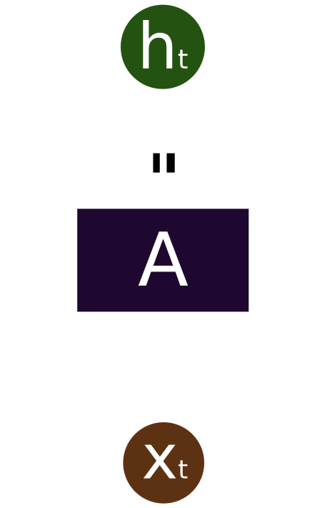
In the above diagram, a chunk of neural network, \(A\), looks at some input \(x_t\) and outputs a value \(h_t\). A loop allows information to be passed from one step of the network to the next.
These loops make recurrent neural networks seem kind of mysterious. However, if you think a bit more, it turns out that they aren’t all that different than a normal neural network. A recurrent neural network can be thought of as multiple copies of the same network, each passing a message to a successor. Consider what happens if we unroll the loop:
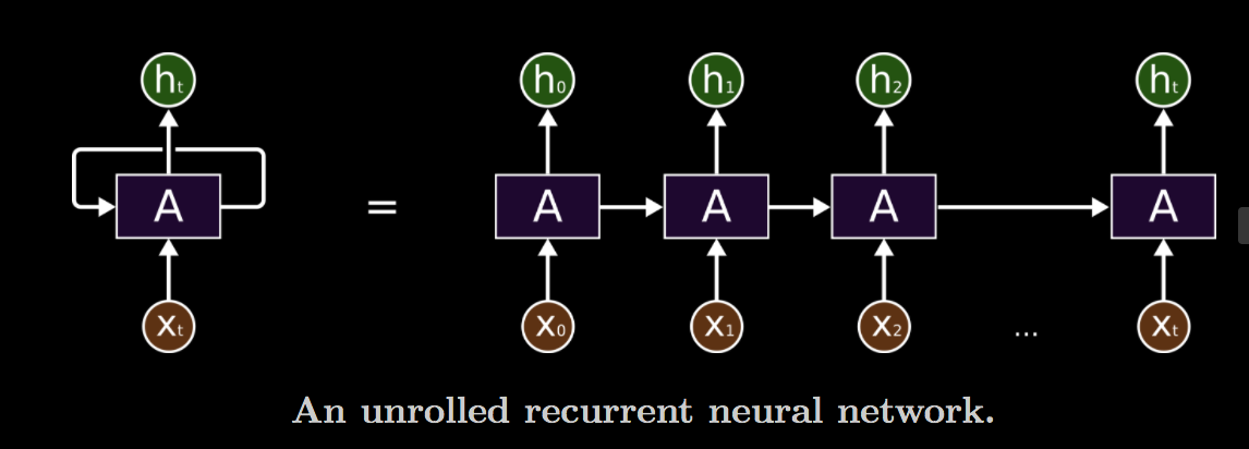
This chain-like nature reveals that recurrent neural networks are intimately related to sequences and lists. They’re the natural architecture of neural network to use for such data.
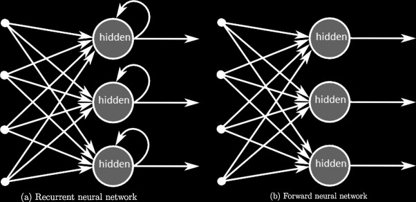
Just for comparison, below is another high level visualization that compares a RNN to a standard Feed Forward Neural Network. Notice how information is fed backwards into each hidden layer. This allows for output from prior timesteps (and as a result, “memory”) to be utilized, and is what makes RNNs great for sequential tasks.
RNN Transformations, Hidden State
Now, let’s zoom in closer on a single neuron, this time with the mathematical operations included. In this diagram, the circle at the center represents a single neuron. This neuron has a hidden state s, which is a vector of numbers representing the current “memory” of the neuron. This neuron is, for the most part, the same as those that we saw in previous lessons: it still has an activation function, and still has weighted inputs. However, as we can see, there is another additional input coming from the previous state of the neuron itself. This is why the neuron is “recurrent”.
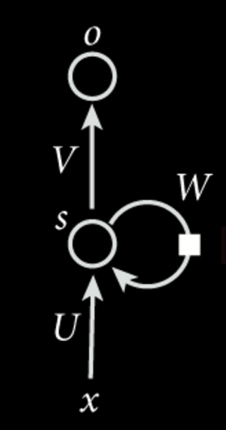
As you can see, previous states of the neuron are “recurrently” fed back through the network via the loop to the right. In this diagram, \(U\) is simply the matrix representing the weights of the new external inputs to the neuron, and serves more or less the same purpose as the weight matrices we saw in earlier neural networks (although this was notated with \(W\) in previous neural networks). You can think of this as deciding what information we should keep from the new input and store in our hidden state \(s\). \(W\) now represents the weight matrix that we use to transform our previous neuron state, and controls what information gets passed onto the next iteration (or timestep) of the network. So, the new state is a function of both our new input and the old state from the previous timestep. Since the old state contains information from all previous timesteps (since it was affected by all previous inputs), the hidden state effectively serves as the “memory” of the neuron.
As an equation, this hidden state update would look like: \(s_t = f(Ux_t+Ws_{t-1}+b)\) where \(f\) is some activation function that we use to squash the values in our hidden state, \(x_t\) is the new input of the sequence at timestep \(t\), \(s_{t-1}\) is the old hidden state, and \(b\) is an optional bias term.
If we want to generate some output from this current state, we apply another transformation matrix \(V\) to our current state, and apply another activation function, giving us our output \(o\).
At each timestep, we use the exact same matrices \(U\), \(V\), and \(W\). Aside from reducing the number of parameters that we need to learn, this also allows this neuron to work on sequential inputs of any length. Instead of having different matrices for each element in the input sequence, each additional element in the sequence simply adds one more timestep to the network.
Unrolled RNN
Looking at our diagram from before, let’s think about what the network would look like over time and how we would actually evaluate it. Once again, we can do this by “unfolding” or “unrolling” the RNN, so that for each node, the previous time input can be clearly be seen as an input to the current node.
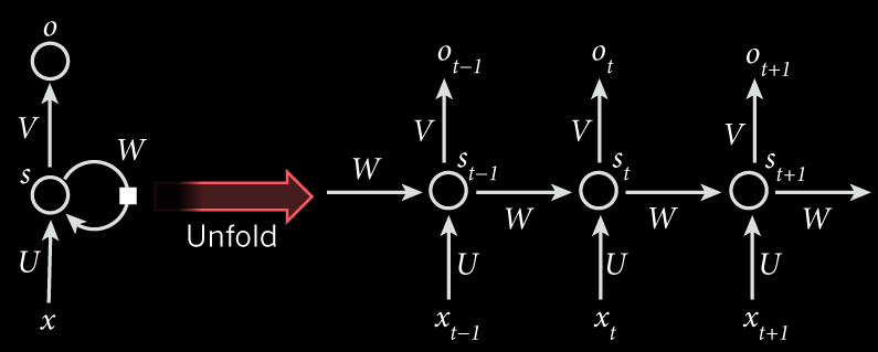
Again, the circles in the diagram are just neurons. However, as time passes and we feed in more and more inputs from the sequence into the network, the state of this neuron changes. We can think of the states of this neuron as the “memory” of the network at time \(t\).
A couple things to note:
- \(x_t\) is the input at timestep \(t\). For example, \(x_1\) could be a one-hot vector corresponding to the second word of the input sentence.
- \(s_t\) is the hidden state at timestep \(t\). It serves as the “memory” of the network, and captures information about what happened in all the previous timesteps. \(s_t\) is calculated based on the previous hidden state and the input at the current timestep: \(s_t = f(Ux_t + Ws_{t-1})\). The function \(f\) is usually a nonlinear activation function such as tanh or ReLu.
- \(s_{-1}\), which is needed to calculate the first hidden state \(s_0\), is typically initialized to all zeroes. So, at each timestep, the neuron transforms the previous hidden state and current input to generate a new output \(o_t\) and part of the input to the next timestep.
- Again, notice that the weight matrices do not change for each iteration. The same weights are used to evaluate an entire sequence.
- \(o_t\) is the output at step \(t\). The above diagram has outputs at each time step, but depending on the task this may not be necessary. For example, when predicting the sentiment of a sentence, we may only care about the final output, not the sentiment after each word. Similarly, we may not need inputs at each time step. The main feature of an RNN is its hidden state, which captures some information about a sequence.
Training RNNs
Although the structure of RNN’s may look intimidating at first, they are actually not very different from regular neural networks. In fact, we can even use the same backpropagation algorithm to calculate the gradient in order to optimise the loss function. Denny Britz provides a nice high level overview for training RNN’s.
“Training a RNN is similar to training a traditional Neural Network. We also use the backpropagation algorithm, but with a little twist. Because the parameters are shared by all time steps in the network, the gradient at each output depends not only on the calculations of the current time step, but also the previous time steps. For example, in order to calculate the gradient at \(t=4\) we would need to backpropagate 3 steps and sum up the gradients. This is called Backpropagation Through Time (BPTT).”
Don’t worry worry if this explanation doesn’t click at the moment – we will delve deep into the details of Backpropagation Through Time in the following sections.
Now that you’ve learned the fundamentals of a RNN, it’s time to look at how different architectures can be used to solve all sorts of tasks!
RNN Usage Example: Language Modeling and Generation
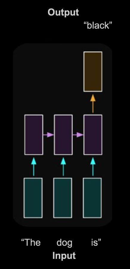
Let’s think about an interesting example. We can view text as just a sequence of words. We can encode each word in our dictionary of words to some vector. We can then train this word level RNN on this sequence of words to predict the next most likely word in a sequence of words. So if we supply some starting text the RNN will be able to predict the next most likely word and we can feed that predicted word back into the RNN to get the next predicted word and so on until the RNN generates enough text. In practice RNNs are able to learn proper English grammar and form complex sentences.
Let’s take a look at the diagram below. The red boxes are the input to the model where each box represents a different word in a sequence of text. In this case, the words “the”, “dog”, and “black” correspond to each of the red boxes. The green boxes are the recurrent layer, which take into account past timesteps as well as the current input. This diagram shows this layer in the “unfolded” or “unrolled” representation.
Lastly, the single blue box represents the output of the model. It makes sense to have only one box here because the output is the prediction of the next word in the sequence.
If you’d like to see some other examples of the flexibility that RNNs provide, take a look at this graphic and caption below from Karpathy’s blog.
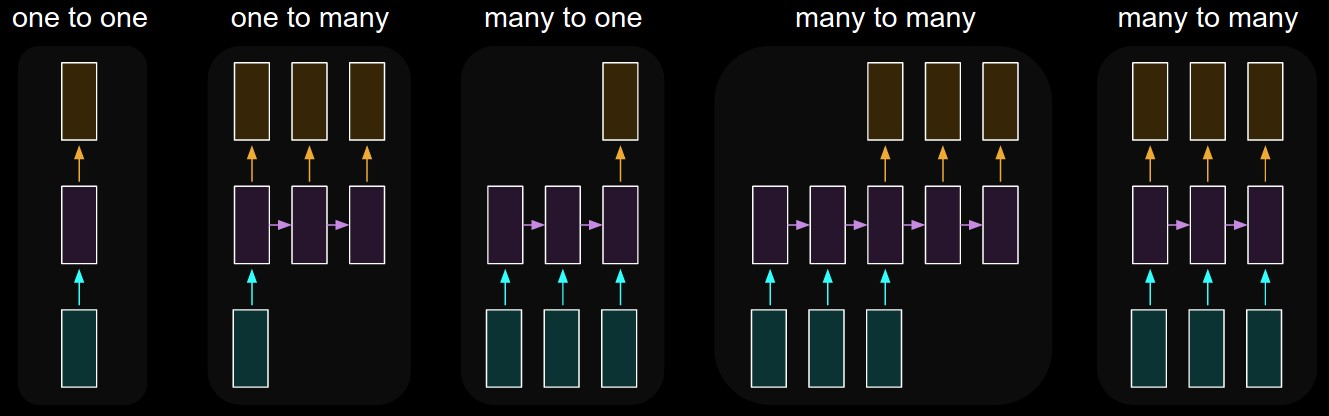
Each rectangle is a vector, and arrows represent functions (e.g. matrix multiply). Input vectors are in red, output vectors are in blue, and green vectors hold the RNN’s state. From left to right: (1) Vanilla mode of processing without RNN, from fixed-sized input to fixed-sized output (e.g. image classification). (2) Sequence output (e.g. image captioning takes an image and outputs a sentence of words). (3) Sequence input (e.g. sentiment analysis where a given sentence is classified as expressing positive or negative sentiment). (4) Sequence input and sequence output (e.g. Machine Translation: an RNN reads a sentence in English and then outputs a sentence in French). (5) Synced sequence input and output (e.g. video classification where we wish to label each frame of the video). Notice that in every case are no pre-specified constraints on the lengths sequences because the recurrent transformation (green) is fixed and can be applied as many times as we like.
Vanishing Gradient, LSTMs
Now that we’ve gone over the basic idea of RNNs, our next step will be to talk about some challenges that we may face when training RNNs in practice, as well as some methods that we can use to overcome these challenges – mainly, a special type of RNN known as a Long Short-Term Memory network, or LSTM for short.
Again, we’ve included both the video of the Karpathy CS231n lecture (a different portion than before), as well as some text and diagram-based explanations. We recommend that you take a quick look at both, and then decide which one you want to go through. If you’re still confused after going through one medium, give the other one a try as well.
(Karpathy actually pokes fun at some of the LSTM diagrams that are out there for their incomprehensibility, but for some of you, the diagrams may be more intuitive than the video. LSTMs can be tough to pick up at first regardless, so you do you.)
Here’s a later portion of Karpathy’s same lecture in which he talks about LSTMs. If you’d like to focus on the video content for this section, you should watch from the 43:30 minute mark until the end. Karpathy starts off by talking about recurrent neurons can be stacked together to form deep RNNs, and then transitions into talking about LSTMs and their various information “gates.” He then explains how LSTMs can manage to overcome a problem that consistently plagues traditional RNNs: the vanishing gradient problem.
At the heart of the LSTM is the cell state, which is analogous to the hidden state that we saw in regular RNNs. LSTMs use a more complex recurrence formula than regular RNNs to manage this cell state, which includes a series of “gates” to control the flow of information through time (e.g. deciding what information to forget from the current cell state, what information to remember from the new input, etc.). This design allows LSTMs to effectively learn and remember long-term dependencies – something that regular RNNs tend to struggle with in practice.
Furthermore, since changes to the cell state rely mainly on additive operations (as opposed to only matrix multiplication), gradients can be more effectively fed back through the network, allowing LSTMs to combat the vanishing gradient problem that tends to come with using backpropagation through time (BPTT).
Backpropagation Through Time, Vanishing Gradient
As mentioned previously, we train Recurrent Neural Networks using the backpropagation through time algorithm, which is very similar to standard backpropagation. The only difference, well is…. time! To help gain some intuition on this process, lets bring back the unfolded RNN diagram from earlier.
Now, let’s replace it with a similar diagram that just rids of some of the labels so that we can get a cleaner look.)
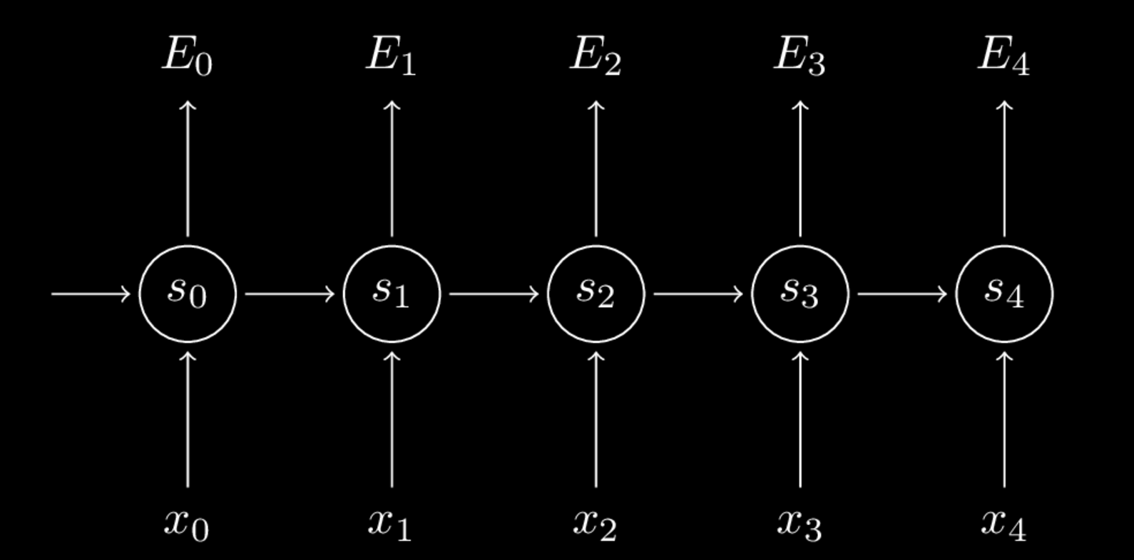
In this diagram, \(o\) has been replaced with \(E\). \(E_t\) is defined below as the cross entropy loss at timestep \(t\), where \(y_t\) is the correct word (or output) at time \(t\), and \(\hat{y}_t\) is our predicted output. \(y_t\) and \(\hat{y}_t\) aren’t included in the diagram, but help determine the cross entropy loss \(E_t\). Their use can be seen in the equations below. Also, in this case, the error is summed up over all previous timesteps because the RNN has multiple outputs corresponding to different timesteps.
\[\normalsize \begin{equation} \begin{split} E_t(y_t, \hat{y}_t) & = -y_t\log\hat{y}_t \\ E(y, \hat{y}) & = \sum_t E_t(y_t, \hat{y}_t) \\ & = -\sum_t y_t \log \hat{y}_t \end{split} \end{equation}\]Since the goal of backpropagation is to find the gradient with respect to each of the parameters, \(W\), \(U\), and \(V\) (if you need recollection of what these vectors represent, refer to earlier in the lesson!). The time aspect of the backpropagation comes into play when a parameter is shared across multiple timesteps. To further understand this process, we will examine specifically the \(W\) vector, which is the weight vector between each neuron at each timestep. The first important insight here is that just as the error was summed across all timesteps, we also sum the gradients at each time step. So,
\[\normalsize \begin{equation} \frac{\partial E}{\partial W} = \sum_t \frac{\partial E_t}{\partial W} \end{equation}\]Now, let’s try to calculate the gradient of \(W\) at a specific time step, say, \(t = 3\). When using the chain rule to compute the gradient with respect to \(W\), we arrive at this equation:
\[\normalsize \begin{equation} \frac{\partial E_3}{\partial W} = \frac{\partial E_3}{\partial \hat{y}_3} \frac{\partial \hat{y}_3}{\partial s_3} \frac{\partial s_3}{\partial W} \end{equation}\]Here \(s_3 = tanh(Ux_t + Ws_2)\). However, since we are dealing with recurrent neural networks, \(s_3\) depends on the hidden states at all previous timesteps. Again, we must sum up the contributions of each timestep in order to find the total gradient, which gives us the equation:
\[\normalsize \begin{equation} \frac{\partial E_3}{\partial W} = \sum_{k=0}^3 \frac{\partial E_3}{\partial \hat{y}_3} \frac{\partial \hat{y}_3}{\partial s_3} \frac{\partial s_3}{\partial s_k} \frac{\partial s_k}{\partial W} \end{equation}\]You can see that we sum up the contributions of each time step to the gradient. In other words, because \(W\) is used in every step up to the output we care about, we need to backpropagate gradients from \(t=3\) through the network all the way to \(t=0\):
Unfortunately, our process is not over yet. We must still account for the fact that \(\frac{\partial s_k}{\partial W}\) yet another application of the chain rule. So, our final equation to represent the gradient of \(W\) would be:
\[\normalsize \begin{equation} \frac{\partial E_3}{\partial W} = \sum_{k=0}^3 \frac{\partial E_3}{\partial \hat{y}_3} \frac{\partial \hat{y}_3}{\partial s_3} (\prod_{j=k+1}^3 \frac{\partial s_j}{\partial s_{j-1}}) \frac{\partial s_3}{\partial s_k} \frac{\partial s_k}{\partial W} \end{equation}\]As you can see, the above equation has the potential to produce a long string of partial derivatives that are multiplied with each other. And when gradients are calculated that involve even more previous timesteps, the chain rule gets longer and longer. This is essentially causes another instance of the vanishing gradient problem (in case you forgot, this occurs because of the small derivatives that certain activations have). Another way to picture this problem is to view the unrolled RNN as a very deep neural network. To find the gradients early on in this unrolled network, we would have to multiply many small chain-rule terms together, resulting in a tiny final gradient. Through this representation, it may be easier to see why the same problem might exist in both cases.
LSTMs
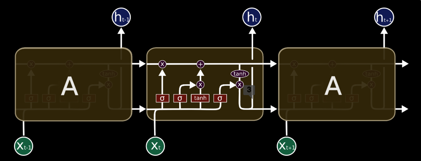
Thankfully, there are various solutions/tweaks that we can apply to the standard RNN structure in order to prevent the vanishing gradient problem. One of the most popular developments is the Long Short Term Memory cell. Most of the information presented in this next section is taken from Christopher Olah’s blog, so the notation is a little different. To get us started with LSTMs, below is the representation for an unrolled RNN that we saw earlier.
Now, the magic of an LSTM network rests in the “memory cells”, which are the boxes labeled \(A\) in the above diagram. The hidden “magic” behind these boxes basically allows the network to “forget” irrelevant information and add/output important and pertinent information through mathematical transformations referred to as “gates”. This capability to more effectively control the flow of information through time brings with it a whole slew of benefits from regular RNNs. LSTM’s have been shown to combat the vanishing gradient problem through use of their “cell state” (explanation soon to follow). Furthermore, most of the work attributed to RNN’s actually use LSTM cells because of their remarkable ability to learn and keep long term information, which regular (“vanilla”) RNNs have been pretty bad at in practice.
For example, let’s say that we are trying to train a RNN to predict the last word in the text: “I grew up in France… I speak fluent French.” Recent information (i.e. “I speak”) suggests that the next word is probably the name of a language, but if we want to narrow down which language, we need the context of “France”, from further back. While RNNs should, in theory, be able to remember past information and handle these long term dependencies, the time gap between this context (“France”) and the desired prediction (“French”) will likely be too much for a regular RNN to handle in practice. That’s where the power of LSTM cells comes into play.
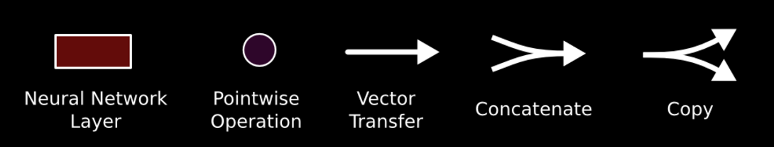
LSTM networks are a special kind of RNN explicitly designed to avoid the long-term dependency problem. For a deeper explanation, we will let Christopher Olah take the reign, since his summary and intuition behind LSTM’s is as clear as it comes and acknowledged throughout the machine learning community. But before we do that, let’s get a handle on the notation of the diagram. Below are of the symbols and their representation.
Cell State
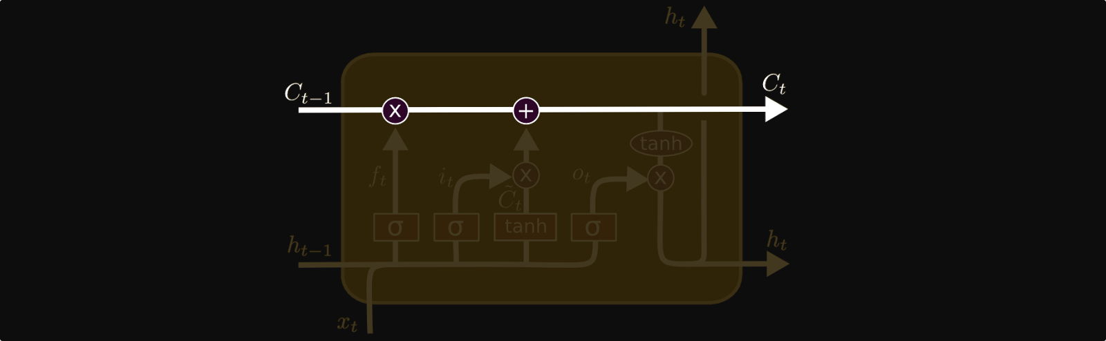
The key to LSTMs is the cell state, the horizontal line running through the top of the diagram. The cell state in LSTMs in analogous to the hidden state in regular RNNs.
The cell state is kind of like a conveyor belt. It runs straight down the entire chain, with only some minor linear interactions. It’s very easy for information to just flow along it unchanged. Also, the process of “adding” information to the cell state (instead of using only matrix multiplications) is what combats the vanishing gradient problem and allows the LSTM to learn long term dependencies.
The LSTM does have the ability to remove or add information to the cell state, carefully regulated by structures called gates. Gates are a way to optionally let information through. They are composed out of a sigmoid neural net layer and a pointwise multiplication operation.
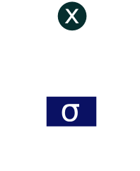
The sigmoid layer outputs numbers between zero and one, describing how much of each component should be let through. A value of zero means “let nothing through,” while a value of one means “let everything through!”
An LSTM has three of these gates, which can be compared to the concept of memory. These gates control what the cell state “forgets” and “remembers” as information is passed along the chain of time by choosing which information gets passed through to the next time step.
Step-by-Step LSTM Walkthrough
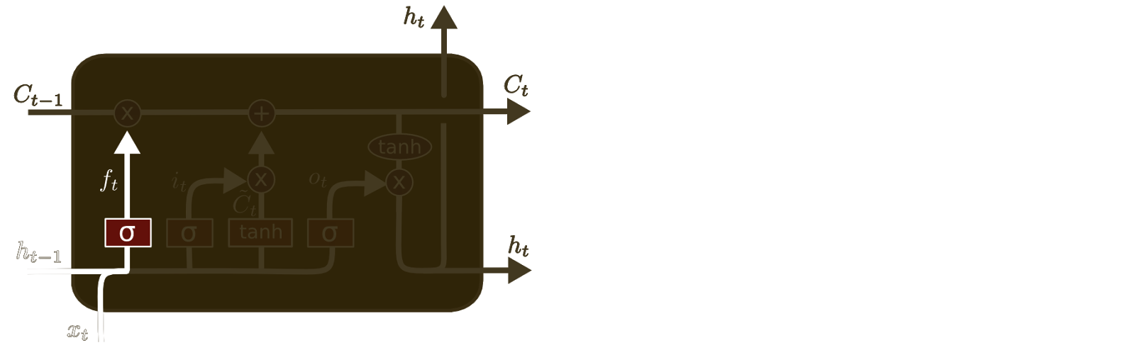
The first step in our LSTM is to decide what information we’re going to throw away from the cell state. This decision is made by a sigmoid layer called the “forget gate layer.” It looks at \(h_{t-1}\) and \(x_t\), and outputs a number between \(0\) and \(1\) for each number in the cell state vector \(C_{t-1}\). A \(1\) represents “completely keep this” while a 0 represents “completely get rid of this.”
Let’s go back to our example of a language model trying to predict the next word based on all the previous ones. In such a problem, the cell state might include the gender of the present subject, so that the correct pronouns can be used. When we see a new subject, we want to forget the gender of the old subject.
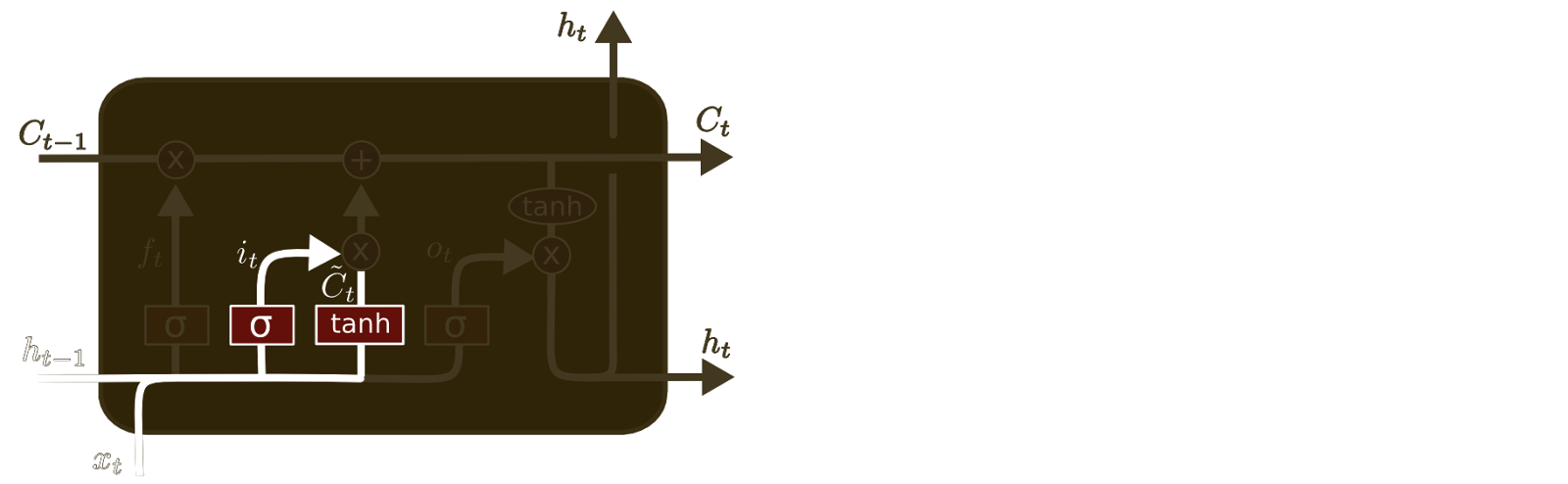
The next step is to decide what new information we’re going to store in the cell state. This has two parts. First, a sigmoid layer called the “input gate layer” decides which values we’ll update. Next, a tanh layer creates a vector of new candidate values, \(\tilde{C}_t\), that could be added to the state. In the next step, we’ll combine these two to create an update to the state.
In the example of our language model, we’d want to add the gender of the new subject to the cell state, to replace the old one we’re forgetting.
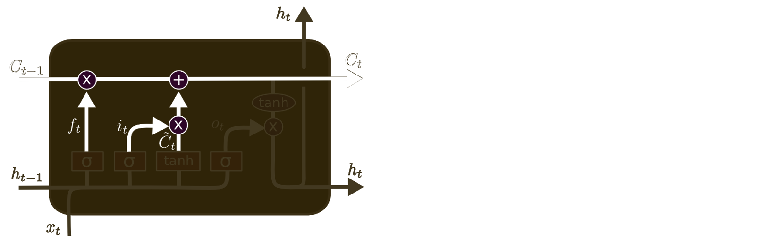
It’s now time to update the old cell state, \(C_{t-1}\), into the new cell state \(C_t\). The previous steps already decided what to do, we just need to actually do it.
We multiply the old state by \(f_t\), forgetting the things we decided to forget earlier. Then we add \(i_t*\tilde{C}_t\). This is the new candidate values, scaled by how much we decided to update each state value.
In the case of the language model, this is where we’d actually drop the information about the old subject’s gender and add the new information, as we decided in the previous steps.
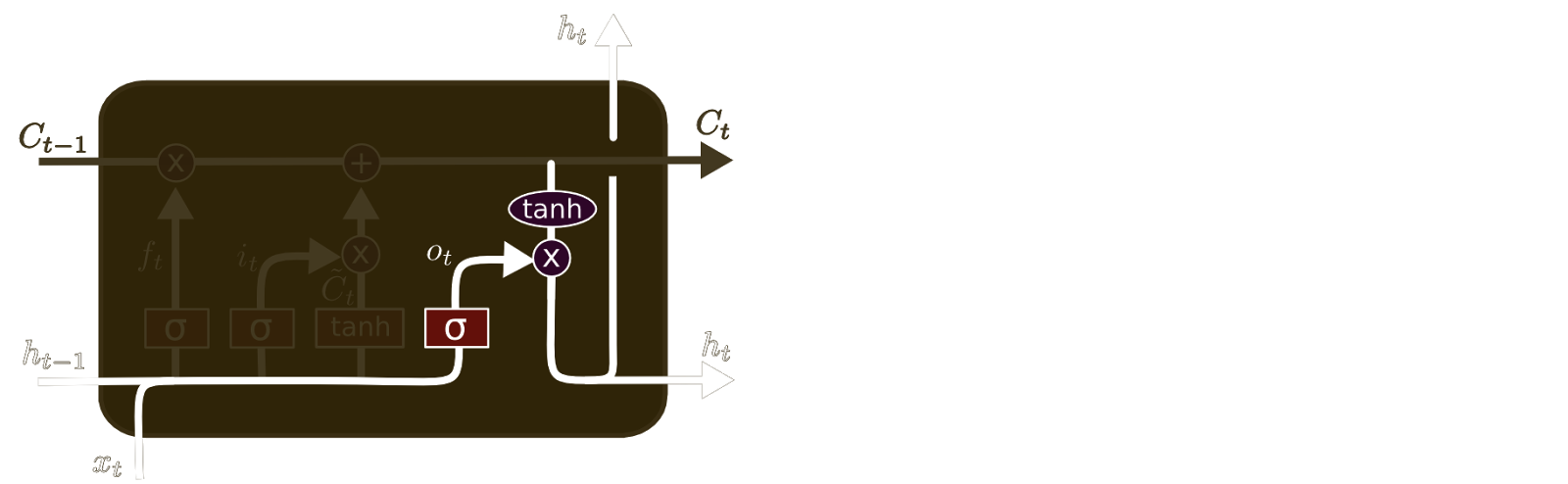
Finally, we need to decide what we’re going to output. This output will be based on our cell state, but will be a filtered version. First, we run a sigmoid layer which decides what parts of the cell state we’re going to output. Then, we put the cell state through tanh (to push the values to be between −1 and 1) and multiply it by the output of the sigmoid gate, so that we only output the parts we decided to.
For the language model example, since it just saw a subject, it might want to output information relevant to a verb, in case that’s what is coming next. For example, it might output whether the subject is singular or plural, so that we know what form a verb should be conjugated into if that’s what follows next.
LSTMs Wrap-Up
Now that you’ve learned the power that LSTM’s behold, you might be wondering “How does one go about using a LSTM?” Well, just as you saw the various creative architectures behind Convolutional Neural Networks, LSTM networks can be constructed in many different ways. Just like how convolutional filters were used to recognize specific patterns in images, input information at each timestep can be fed into multiple LSTM units at once as well.
The theory behind this is also similar to CNNs; each LSTM unit can be trained to recognize and remember specific information based on the inputs. (If we’re looking at textual inputs, then one unit could learn to detect quotations, while another could learn to detect new lines and paragraph breaks.) Then, the information accumulated by these units can be connected to series of dense layers in order to condense and extract information that is most input to the final output.
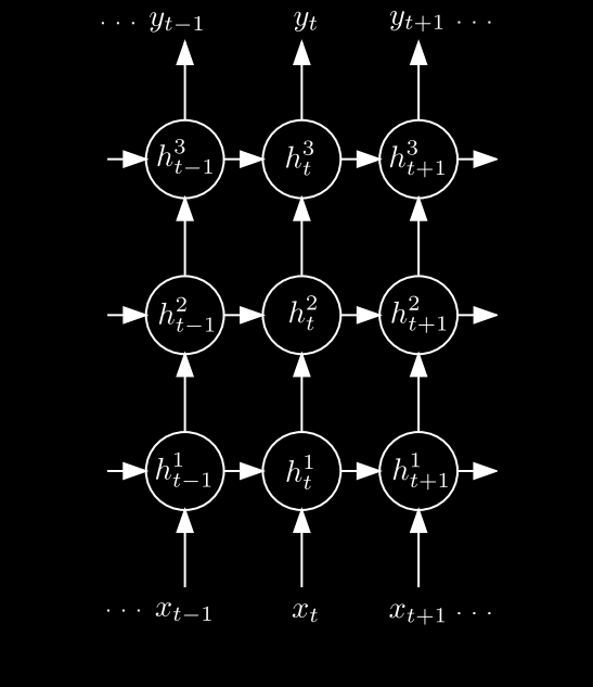
Another common approach is to build “deep” LSTM networks, in which layers of LSTM’s are “stacked”(again in a very similar manner to standard deep neural networks) in order to build more complex representations of the data passed through the network. This diagram (that we saw earlier) shows how multiple units can be visualized together.
Having seen some of these approaches, the bottom line is that research dealing with RNN architectures is constantly evolving as more and more successful solutions are found. For example, a recent trend has involved “attention” mechanisms that essentially let the RNN pick specific aspects from a pool of past information. Xu, et al. (2015) and “Attention is All You Need” (2017) provide good insight into this new research direction. The bottom line is to stay updated! Research within RNN’s and the machine learning field as a whole is progressing rapidly, providing great insight for many pertinent problems.
Applications in Society
Just as we saw with convolutional neural networks, RNNs have been used in a variety of real world applications related to processing sequential data. To give just a few examples:
- Language: [Connecting the world via machine translation], [More effective speech recognition]
- Social Media: [Sentiment Analysis on Tweets]
- Transportation: [Training self-driving cars to predict pedestrian trajectories and avoid collisions]
- Media: [Automatic video captioning], [Image captioning]
Main Takeaways
- RNNs are designed to work on sequential inputs, and allow for a lot of flexibility in architecture design.
- RNN neurons maintain an internal hidden state which serves as “memory.” Since the hidden state is a function of the current input in the sequence and the hidden state at the previous timestep, it contains information from all previous timesteps.
- In practice, regular RNNs (1) cannot handle long-term dependencies and (2) suffer from the vanishing gradient problem, so LSTMs are usually used instead.
- LSTMs manage their cell state by using a variety of “gates” to more effectively control the flow of information through time, which allows them to learn and remember long-term dependencies and combat the vanishing gradient problem.