Introduction
If you have heard of machine learning before, chances are you have heard of neural networks as well. Neural networks are often called artificial neural networks because their structure is loosely modeled off of the structure of the brain. The human brain contains around 100 billion neurons. Each neuron is a small cell that transmits signals, and is connected to other neurons via their synapses. These small neuron units and their connections when linked together give humans the capability to think.
A similar approach was taken in developing artificial neural networks. In an artificial neural network, many units (artificial neurons) function together to give the system the capability to learn from data. Like the brain, these neurons are connected to each other. The exact structure of neural networks and how these connections and neurons work will be discussed in the following pages.
So why are neural networks so popular? In recent years, neural networks have exploded in popularity. Cheaper and more powerful hardware has allowed researchers to link together thousands, and even millions, of artificial neurons into artificial neural networks, allowing for a more powerful extension of machine learning called deep learning. This renaissance in deep learning has seen countless breakthroughs in neural networks and their applications. The second reason is the versatility of neural networks. With their highly flexible architecture, neural networks have found applications in text, speech, images and much more. They have proven to be a useful machine learning tool in a variety of situations.
For better or for worse, there is a good amount of math associated with neural networks. This post will discuss much of the surface level theory that goes into a neural network. From this theory, you should gain a good understanding of how basic neural networks work, which will then allow you to work on actual implementations.
Since the material in this lesson may be more challenging than in previous lesson, we have included both video and written content. We recommend that you watch the video first and then read through the writtent content, since it will reinforce your understanding of the video. As usual, take your time if necessary, some of these ideas are challenging and may take a few read-throughs to really sink in.
Intro to Deep Learning
Before we delve too deep into the theory behind neural networks, it may help to discuss how neural networks, which are the key enabler of deep learning, relate to linear and logistic regression. Neural networks are more flexible than simple linear regression. As we will see, the structure of neural networks result in a more complex analysis of our input data. To be more specific, neural networks consider the combinations of features, which are often just as important as the features themselves when making a hypothesis. Using the same housing prices example as last time, a house with 2 bedrooms and 2 bathrooms may be an influential factor in the sale price. Linear and logistic treat these features separately; they compute how each individual feature influences the sale price (denoted by the weights) and sums them together to make the hypothesis. But neural networks will consider combinations of features, in addition to the features themselves. To help visualize this, take a look at the general structure of a neural network:
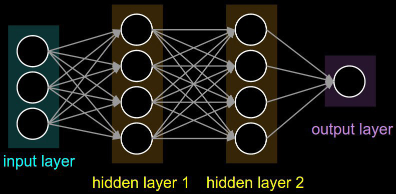
After the input layer, each successive layer of neurons learns to detect some increasingly abstract combinations of features from the previous layer, until we finally use these learned compound-features to make a final prediction.
This layering of features may not seem too groundbreaking right now, but you’ll eventually see how this concept of learning more and more abstract combinations of features will allow us to build up representations of much more complex types of data, such as images, text, etc.
Neural Network Architecture
Let’s start with a video. Try your best to gather a conceptual understanding at this point, the written content will cover everything in a little more depth.
At a completely abstract level, a neural network just takes in some inputs (e.g. the brightness of each pixel), applies some transormations, and then generates an outputted prediction (e.g. the number). It really is just a big, complicated function.
Between the input and output layers, we also have some hidden layers made up of neurons. Each neuron takes in the output from the previous layer, scales each piece of input data by some weights (much like in linear/logistic regression), sums up over these weighted inputs, adds a bias and then applies an activation function. This final activation then gets passed to the neurons of the next layer as a new series of inputs. The next couple of sections will get into what exactly it is the neuron does.
Networks
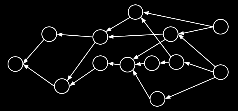
What is a neural network? Let’s begin by dissecting the name itself. In mathematics, a network can be thought of as a graph, and is nothing more than a set of vertices or nodes that are connected via arrows, or edges. They can be used to represent everything from connections within friend groups (mathematical “social networks”) to connections between artificial neurons. In our neural network the nodes and edges will have special meanings. An example of a network is shown here.
The other important aspect of our neural network is, of course, the “neuron.” We want our network to be able to understand and learn. While this might seem difficult at first, we will see that neural networks use these graphs as a powerful structure to define operations to learn desired responses. The building block of these networks is the neuron.
The Neuron
Before we talk about full neural networks, let’s examine an individual artificial neuron. An illustration of an artificial neuron is shown below.
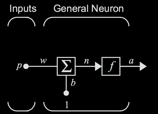
Before we get into the actual intuition of what a neuron is, let’s get through the math behind one, since the artificial neuron is at its core a mathematical construct.
The input of the incoming edge is notated as the scalar \( p \). This edge has a scalar weight \( w \). The weight is multiplied by the input to form the value \( wp \). This is then sent into the the summation block, which sums the input \( wp \) and the bias \( b \). Notice that the bias has no dependence on the input. Summing these two terms together then gives the weighted sum \( wp + b \), which we will represent as \( n \).
The output of the summation \( n \) is then passed through the activation function \( f \). The activation function is just some real valued scalar function that we use to squash our output to within a desired range. This then gives the final output of the neuron, \( f(n) = a \). The neuron output can then be calculated as: $$ a = f(wp + b) $$
Neuron Intuition
So what is the intuition behind a neuron? We can view the output of this neuron as making a decision. This decision is based on the inputs, weights and bias of the neuron. Suppose you are trying to make the decision of if you want to go to a party tonight. Let's say we live in a world where this decision depends on only two factors: 1. if you are tired (\( x_0 \)), and 2. if your best friend at the party (\(x_1\)). Note that these factors are simple yes or no questions. We can encode a yes as \( 1 \) and a no as \( 0 \).
The importance of these two factors will vary a lot from person to person. This corresponds to different weight values. For this neuron, say that our activation function is the simple linear function \( f(x) = x \), and that any output \( > 0 \) means we should decide to go to the party and any output \( < 0 \) means that we should decide to not go. A normal person would not want to go to a party while tired. We should then make the weight (\(w_0 \)) for the "are you tired" input (\( x_0 \)) negative. On the other hand, you would hopefully want to go if your best friend is going, so the corresponding weight (\(w_1\)) for that input (\(x_1\)) would be positive.
Say that you absolutely hate going out when you are tired and this is far more important than your best friend being at the party. We could make \( w_0 = -10 \) and \( w_1 = 1 \) to represent this. If you are tired, you will never go out even if your best friend is there, because \( -10 + 1 < 0 \). However, if your best friend is there but you are not tired, you would still go out, because \( 0 + 1 > 0 \). If you were not tired and your best friend wasn't there, you would be right on the decision boundary and could just choose randomly.
Now that we have an idea of a decision boundary set up, we can now incorporate bias to change our decision boundary. When we had no bias in the previous example, the decision boundary (or cutoff) was 0. If someone is more or less inclined to go to parties no matter what the inputs are, we can account for this by adding on a bias term \( b \) to the weighted sum \( w_0x_0 + w_1x_1 \), thereby shifting the decision boundary. A more positive bias means that we are more inclined to go to parties given any inputs.
To demonstrate, let's change the problem slightly by making \( x_1 \) the number of your friends that are going. If you generally enjoy going to parties, your decision neuron could have \( b = 2 \), and of course you do not like going to a party while tired but would be more inclined to go if you had more friends there, so \( w_0 = -4, w_1 = 1 \). So even if you are tired, it would only take three of your friends to be there for you to want to go to the party (\( (-4*1) + (1*3) + 2 = 1 \)). But if \( b = 0 \), it would take five friends if you are tired (\( (-4*1) + (1*5) + 0 = 1 \)).
Activation Functions
In our example, we chose the linear activation function, where our equation took the form \( a = w_0 x_0 + w_1 x_1 + b \). This means that our output activation \( a \) could be any real number, positive or negative. Our simple linear linear activation function would look like the below for input \( p \) and output \( a \).
![]()
However, there are a variety of other activation functions that are employed in neurons giving different ranges of responses.
Going back to the decision about the party, say there is another person that is trying to predict if you are going to go to the party. In this case, we would want our output to be a **probability** (between 0-1), so our earlier cut-off rule will not apply. We could just take the pure score value, and based on how positive or negative it is, determine how certain you are to go to the party. However, there is a function called the sigmoid function that does a better job of representing these probabilistic outputs. Any probability can be represented between 0 and 1. The sigmoid function does just this, by squashing any real value to fit between 0 and 1. Below is an image of the sigmoid function in action.
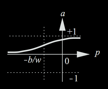
After applying the sigmoid function, very negative values (which, using our previous cutoff rule, would make us not want to go to the party) will produce values close to 0; very positive values (which would make us want to go to the party) will produce outputs close to 1.
Neural networks are probabilistic systems, and therefore functions like the sigmoid function are a lot more powerful than just the linear activation function. We will see why the sigmoid function and other non-linear functions are so powerful in later lessons.
Forward Propagation
Now, let’s start chaining multiple of these neurons together and start formalizing and abstracting the math behind the networks. Watch the following video for some intuition on how the complete process of stacking layers of neurons on each other works. Forward propagation simply refers to the process of propagating an input through all the neural network layers in order to evaluate the final output. This idea was introduced in the video above, but this one will allow us to take a closer look.
Before training the model, we must decide on some hyperparameters for our model: these include values like the number of hidden layers in our network, how many neurons will be in each hidden layer, etc. The actual automated learning process takes place in the weights of the network, which are similar to the model weights that we saw in linear/logistic regression. We can perform the data transformations described above by placing these weights in a matrix, and then multiplying the input matrix by this weight matrix. The result is then fed through our activation function to squash the values to within our desired range, finally giving us the outputs of the hidden layer. To get from our hidden layer to our final prediction, we once again multiply the outputs of the hidden layer by our last weight matrix and apply our activation, giving us a final prediction that lies within our desired range.
- This process is called “Forward Propagation” because we start with our input data \(X\) and propagate it forward through the layers of our network, applying matrix multiplications and activation functions until we end up with our final result, \(\hat{y}\).
- Since we started with random weights and haven’t yet trained our network, this neural network is still pretty much useless in generating meaningful outputs. In the next lesson, we’ll see how we can train a neural network so that it can start to have meaningful outputs.
Once again, we’ll be measuring the error of our network using a cost function, and applying our good friend gradient descent on the weights of our neural network to minimize this cost function. The goal is that after optimizing our model weights, propagating our inputs (e.g. hours slept, hours studied) forward through the network will cause the input data to become transformed in such a way that the network outputs a reasonable final result (e.g. predicted test score).
Vector Formulation
Before moving on, let's clean up some of the math behind what we have developed with the neuron so far. Say we have the multiple input neuron pictured below.
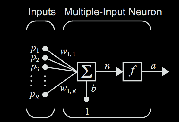
Each of the inputs to the node can just be represented as a vector to make the representation easier. $$ \textbf{p} = \begin{bmatrix} p_1 \\ p_2 \\ p_3 \\ \vdots \\ p_R \end{bmatrix}$$ (We'll use bold face to represent vectors.)
Likewise, we can also formulate the list of weights for each input value as a vector. $$ \textbf{w}_1 = \begin{bmatrix} w_{1,1}, w_{1,2}, w_{1,3} , \dots w_{1, R} \end{bmatrix} $$ The first subscripted number represents the neuron number (which is 1 because we only have 1 neuron), and the second subscripted number represents which input the weight corresponds to. Note that the weight vector is a row vector (not a column vector); due to the way matrix/vector multiplication works, this will become necessary for when we will have to multiply this weight vector with the input vector.
Just as before, we are simply multiplying the inputs by their corresponding weights. So our next step would be just to multiply each input in the input vector by the corresponding weight in the weight vector. $$ \begin{bmatrix} w_{1,1} p_1, w_{1,2} p_2, w_{1,3} p_3, \dots w_{1,R} p_R \end{bmatrix} $$
The next step is to go through the summation. Summing up the components of this vector gives $$ w_{1,1} p_1 + w_{1,2} p_2 + w_{1,3} p_3 + \dots + w_{1, R} p_R $$
This is the same as just multiplying the two vectors \( \textbf{w}_1 \textbf{p}\). Then we add in the bias \(b\), which, as before, is just a single scalar. $$ n = w_{1,1} p_1 + w_{1,2} p_2 + w_{1,3} p_3 + \dots + w_{1, R} p_R + b = \textbf{w}_1 \textbf{p} + b$$
Note that this entire expression \(n=\textbf{w}_1 \textbf{p}+b\), which represents the weighted sum of all the neuron's inputs (including a bias), is still just a scalar. (In the forward propagation video, this scalar was represented as \(\textbf{z}\).) This is because \(\textbf{w}_1\) is a \(1 \times R \) matrix, while \( \textbf{p} \) is a \( R \times 1 \) matrix, resulting in a \( 1 \times 1\) matrix. We then squash this weighted sum using the activation function to get the final output of the node. $$ a = f(\textbf{w}_1 \textbf{p} + b )$$
This one equation pretty much sums up everything that a single artificial neuron does: multiplying the neuron’s inputs by their corresponding weights, summing up these weighted inputs (along with a bias term), and then applying an activation function at the end to squash the output to within a desired range.
The next step is to see what happens once we start working with multiple neurons, which we can combine vertically to form layers. We will first look at the case where we have just one layer of neurons.
Layers of Neurons
We know that the weights of a neuron control how a decision is made by the neuron. Different weights will give a neuron different decision properties. What if we wanted to work with multiple neurons, each with different weights at the same time? In this case, each neuron can be thought of as making some different decision based on the same inputs (e.g. whether to go to the party, what to bring to the party, etc.). We could do this by stacking the neurons into a layer of neurons, where the inputs are fed into each neuron in parallel.
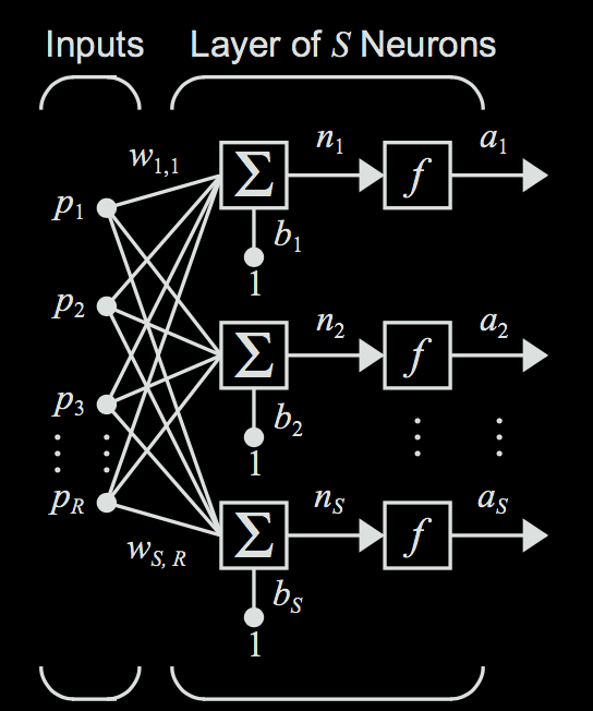
Now, the same principle applies as before: only now that we have multiple neurons, each neuron will have its own weight vector \(w_i\). Each neuron will use its own weights to generate a different output \(a_i\) .
For neuron \(i\), calculate the output \(a_i\) through the following formula. Note that we are assuming that all of the neurons are using the same activation function, which is a safe assumption to make for this case. $$ a_i = f(\textbf{w}_i \textbf{p} + b) $$ However, we can compact this further, and view the weights as a matrix of weights represented as follows. Let's say that there are \(S\) neurons (or nodes) that the input is being fed into. Each row in the matrix represents all the weights for one given neuron. Each column represents the weights used by different neurons for one given input feature. $$ \textbf{W} = \begin{bmatrix} w_{1,1} & w_{1,2} & w_{1,3} & \dots & w_{1,R} \\ w_{2,1} & w_{2,2} & w_{2,3} & \dots & w_{2,R} \\ w_{3,1} & w_{3,2} & w_{3,3} & \dots & w_{3,R} \\ \dots & \dots & \dots & \dots & \dots \\ w_{S,1} & w_{S,2} & w_{S,3} & \dots & w_{S,R} \\ \end{bmatrix} = \begin{bmatrix} \textbf{w}_1 \\ \textbf{w}_2 \\ \textbf{w}_3 \\ \vdots \\ \textbf{w}_S \\ \end{bmatrix} $$ When we multiply this weight matrix by the input vector (\(\textbf{Wp}\)), we will get a vector representing the weighted sums for each neuron in this layer.
Next, since there are now multiple neurons each making different decisions, we will have one bias term for each of our \(S\) neurons. We can represent these with a bias vector (\(\textbf{b}\)), which will then be added on to our vector of weighted sums. $$ \textbf{b} = \begin{bmatrix} b_1, b_2, b_3, \dots b_S \end{bmatrix} $$
Finally, we can get our vector of outputs (or activations) \(\textbf{a}\) by passing each value of the vector through the activation function. $$ \textbf{a} = f(\textbf{W} \textbf{p} + \textbf{b})$$ This then gives us a vector representing the final outputs for each neuron in the layer.
Multiple Layers
What happens if we feed the outputs of one layer of neurons into another layer of neurons?
This is where we begin to see the power of neural networks. Each layer of neruon works on the abstraction of the previous layer. This allows deeper layers to make more complex and higher level decisions. Let's take a concrete example. Say you were builidng a neural network that takes as input handwritten images, just like in the first video. The first layer could detect edges. The second could identify the contour the edges form. The third could take these contours and identify them with shapes. The fourth and final could take these shapes and associate them with numbers.
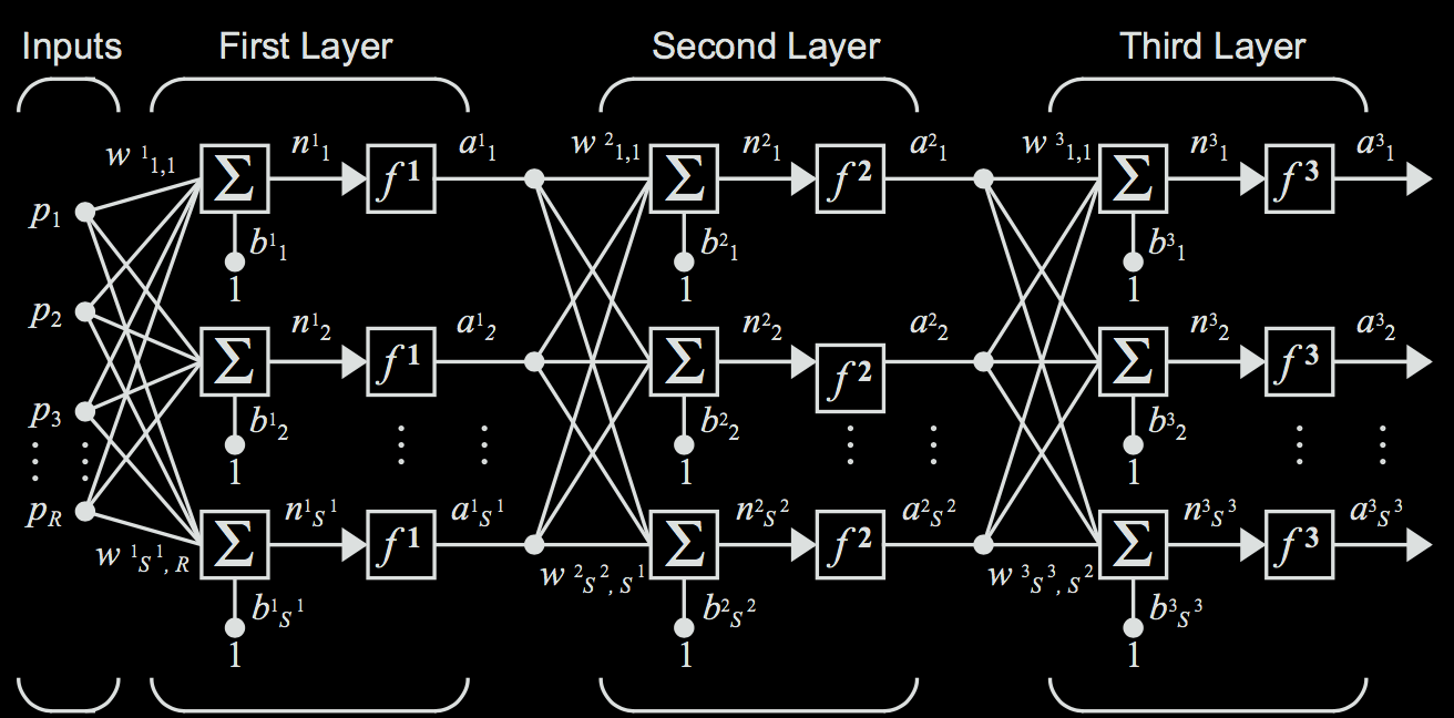
Now, notate the weight matrix for layer \(i\) to be \(\textbf{W}^{i}\), and the corresponding bias vector for layer layer \(i\) to be \(\textbf{b}^{i}\). Note that the number of neurons in each layer can differ. The neurons in any given layer are connected to all of the neurons in the neighboring layers, so the exact number of neurons in the neighboring layers doesn't really matter. The example below is a more concrete depiction of such a network.
We can simply use the rules used to compute the output of one layer and extend it to multiple layers. In this case, the output of one layer will be fed in as the input to the next layer, resulting in a composition of functions that sort of resembles a sandwich when written out completely. For instance, to compute the output of the above 3-layer network, you would evaluate the following equation. $$ \textbf{a}^3 = f^3 ( \textbf{W}^3 f^2 ( \textbf{W}^2 f^1 (\textbf{W}^1 \textbf{p} + \textbf{b}^1) + \textbf{b}^2) + \textbf{b}^3 ) $$ Notice how the input \(p\) is propagated from the left of the network to the right of the network.
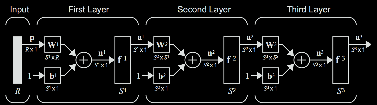
Typically, you will see neural networks illustrated in the less expressive version shown below to save space. In this illustration, each node simply represents one neuron.

Conclusion
That is all for the basics of neural network building blocks. You should be able to see how a neural network produces an output from some input. But what are all these transformations doing? The key is choosing the right values for the weights and the biases to make the network do interesting things. We can do this through having the network learn the weights and biases.
We simply tell the neural network to learn, for some datset \(X, Y\), the mapping from \( X \) to \( Y \), and the network will find the appropriate weights to do so. To go back to our party example, we would feed the network a bunch of examples of times you have decided to go (or not to go) to parties, along with the inputs from each instance (were you tired or not, how many of your friends were there), and the network would be able to learn the correct weights so that it could predict if you would want to go to a certain party or not given some new inputs.
When it comes down to it, the neural network is still a statistical learner: given a set of input data \(X\) and a set of output data \( Y \), a neural network can learn a reasonable mapping from \( X \) to \( Y \). Thanks to the power of deep learning, it just so happens that the mappings neural networks generate can be much more powerful than those generated by linear or logistic regression.
References
- http://neuralnetworksanddeeplearning.com
- https://hagan.okstate.edu/NNDesign.pdf
- https://www.amazon.com/Deep-Learning-Adaptive-Computation-Machine/dp/0262035618
- https://cs231n.github.io/
- https://jamesmccaffrey.wordpress.com/2013/11/05/why-you-should-use-cross-entropy-error-instead-of-classification-error-or-mean-squared-error-for-neural-network-classifier-training/