Introduction
Many machine learning models require large training sets to optimize their performance. While the results can exceed previous statistical models and even human performance, these datasets are often expensive and time-consuming to curate. The solution? Transfer learning. This machine learning strategy is based on the concept of transfer. Essentially, transfer is a general term for when people utilize previous experience to learn new tasks. For example, a violinist learning the piano may draw from their prior knowledge in rhythm, phrasing, and musicality to improve their piano skills. Consequently, this person may have an advantage in learning piano over people with no musical background.
![]()
In ML, we use transfer to boost the performance of a model with a different one that was optimized for a similar task. Ultimately, the goal is to increase the learning rate and overall accuracy of the target model while avoiding the need for a large, labeled training dataset.
![]()
Since the general transfer concept is broad, transfer learning methods widely vary depending on the problem. This article will break down commonly used transfer learning methods, but it is by no ways a comprehensive review. If you want to dive into other topics including heterogenous transfer learning, online transfer learning, and lifelong transfer learning, please check out the further reading below. Additionally, this blog will explain concepts behind each method rather than diving into the math. If you are interested in the specifics of a particular method, please read the original paper for that particular method.
Most popular machine learning frameworks offer approaches that use frozen layers of pre-trained models as a base for new models. This is a very common type of transfer learning called parameter control (inductive learning). In this blog, we will briefly discuss this method and will also describe other transfer learning techniques beyond parameter control.
Formal Definition
Before diving into the formal definition of transfer learning, let’s cover some basic terms.
First, we distinguish between source and target. The source refers to the model where learning is transferred from whereas target refers to the model that you are transferring learning to improve performance.
Here, we are using model quite loosely. But in general, a model encompasses two parts: domain and task.
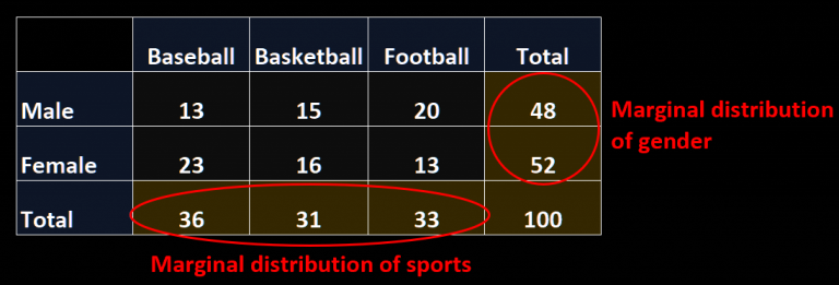
You can think of the domain as your dataset. The domain contains a set of attributes. If you were measuring heart disease across the United States, you might measure features like your body mass index (BMI), heart rate, or cholesterol levels. These features are defined as the feature space, \(X\). Another important term in defining the domain is the marginal distribution, \(P(X)\), which describes the distribution of a single feature in the dataset. “Margin” refers to the literal margin where statisticians would sum the number of instances with a particular attribute.
Task, on the other hand, could be thought of as your goal. It consists of the label space, \(Y\), and the implicit decision function, \(f(x)\). The label space is the set of categories you are classifying different samples of your dataset as. Taking the heart disease example again, the label space might consist of two attributes “high risk” and “low risk.” The implicit decision function maps all domain instances to their respective labels within the label space. All predictors aim to approximate the implicit decision function.
With some terms defined, let’s talk about the formal definition of transfer learning. To better understand the nuances between each transfer-learning method, it’s important to contextualize the approach with the formal definition:
Given a source domain \(D_{S} = \{ X_{S},\ {P(X_S)}\}\), the source task \(\mathcal{T}_{S} = \{ Y_{S},\ f_{S}\}\), the target domain \(D_{T} = \{ X_{T},\ {P(X_T)}\}\), and the target task \(\mathcal{T}_{T} = \{ Y_{T},\ f_{T}\}\), such that \(\mathcal{T}_{T}\ \neq \mathcal{T}_{S}\), optimize the target predictive function \(f_{T}\) on \(D_{T}\) using knowledge about source domain and source task.
This definition summarizes the above section in mathematical terms and describes the class of transfer learning algorithms. Each method distinguishes itself by how it optimizes the target predictive function.
Organizing the Problem
Before diving into specific methods, let’s break down and organize the overall common approaches to transfer learning.
Space-Setting Categorization
Transfer learning problems can be divided into two main categories: homogenous and heterogeneous.
Homogenous methods are applied to problems where both the source and target domains have the same feature space. These models assume that the domains only differ with the marginal distributions. For instance, if you are looking at disease patterns in two different cities, the datasets will have the same types of features, including demographic and outbreak data. The only difference in the domains is the marginal distribution. In this case, the divergence in marginal distribution is driven by locational, economic, and political differences between the cities. Homogenous transfer learning adapts the domains by correcting the differences in data distribution.
A heterogeneous problem is when neither the feature set nor marginal distribution is the same. In addition to distribution adaption, these methods will also correct for feature space adaption. A successful example of heterogeneous transfer learning is utilizing text document classification to enrich image classification for social media posts. Since heterogeneous methods must address differences in both the source and target domains, they are considered more complex problems.
In general, this blog post only covers methods that solve homogenous problems.
Label-Setting Categorization
Another consideration when constructing a transfer learning problem is label availability in source and target domains. There are three categories, ranked in terms of difficulty:
- Inductive transfer learning: both labeled source and target domain instances
- Transductive transfer learning: only labeled source domain instances
- Unsupervised transfer learning: neither source nor target domain instances are labeled
Caveats
Is it possible that transfer learning can make our target model worse? Absolutely! Returning to the violinist example, one could speculate that not all skills learned in violin playing will transfer 1:1 to piano playing. For example, playing the violin requires specific hand positioning and posture. These habits could negatively impact piano playing which require a different set of hand positionings. In this case, violin experience may slow down learning the piano. In transfer learning terms, this is called negative transfer. The informal definition of negative transfer is “transferring knowledge from the source can have a negative impact on the target learner.” More formally, the problem satisifies negative transfer when the inclusion of the source domain and task increases the expected loss. The following factors all contribute to negative transfer:
The degree of similarity between source and target domains
If the domain distributions are too different, the divergence will be too great for meaningful transfer.
How well knowledge is transferred between domains
Method selection may drive whether such knowledge can be transferred.
Ratio of labeled target data to source data
Decreasing the amount of labeled target data will lower the chance of negative transfer since the target model will perform poorly on fewer instances of labeled data. However, this approach could result in a weak model. Increasing the amount of labeled target data may improve performance, but an overabundance of labeled data will exacerbate the difference between source and target domains.
With these factors in mind, it is vital to choose a transfer method that can leverage the labeled target instance to mitigate overall differences between the source and domain. Proposed models to avoid negative transfer reweigh source samples to increase the similarities between source and target domain (e.g. Discriminator Gate). We’ll discuss the various methods commonly employed. In general, these methods are divided into data-based and model-based approaches.
Data-Based Approaches
Data based approaches generally adjust the target and / or source data to deal with the divergence in distributions. We will briefly cover the theory behind each technique. If you’re interested in learning more about any method, you can read more about them in the sources!
Instance Weighting
Weight source-domain instances in the loss function to reduce differences between marginal distribution (similar to mitigating negative transfer). This strategy is particularly useful when transferring between demographic shifts (elderly versus youth individuals, warm versus cool climates).
\[{\min _{f}}{\dfrac {1}{n^{S}}\sum _{i=1}^{n^{S}}{\beta _{i}\mathcal {L}\left ({f({x}^{S}_{i}),y^{S}_{i}}\right)}+\Omega (f)}\]This equation is minimizing the overall loss of the source task weighting by across all instances. \(S\) denotes source, \(f\) is the decision function, \(\mathcal {L}\) is the loss function, \(n^S\) is the number of instances in the source, and \(\Omega(f)\) is the structural risk of the decision function. \(B_{i}\) denotes the weighing parameter, which is what instance weighing models attempt to obtain since it is the theoretical ratio between target and source marginal distribution.
Feature Transformation
Feature transformations translate instances from source domain into instances from target domain. There are several advantages to feature transformation:
- Minimizes distribution differences
- Preserves data structure
- Finds relationships between source and target features
There are three general types, and many feature transformation algorithms will include elements from all of the below types:
- Feature augmentation: Alter feature space to include general, source, and target features and train on transformed labeled instances
- Feature reduction: Distill instances into the most critical features with dimensional reduction to find a more abstract representation of the original features. This could be done by mapping, clustering, or encoding.
- Feature alignment: Align distribution features of source and target.
Model Based Approaches
In this section, we’ll briefly cover common approaches that alter the model to improve target prediction.
Parameter Sharing
Like the name implies, parameter sharing refers to transferring the parameters of the source model to the target model and is commonly employed for transfer learning in neural networks. Even if you aren’t too familiar with transfer learning, you are most likely aware of parameter sharing approaches. Since machine learning models optimize parameters during training, the knowledge of the model can be represented by the parameters themselves. Parameter sharing can be done in multiple ways, including injecting the parameters of a pretrained model to a target model or fine-tuning the final layers of a network with a frozen pre-trained encoder.
Model Control
Aside from leveraging parameters, the objective function can be modified so that source model knowledge can be transferred during training. As a reminder, the objective function is optimized during training to assure your model correctly achieves its goal. Domain adaption machine (DAM) is a framework to establish transfer through the objective function with the addition of regularization terms, which control the complexity of the model to avoid overfitting. Other works have expanded on this approach by developing different regularizers that employ transfer between the source and target model.
Model Ensemble
Before, we’ve only discussed methods with one source model. Yet, in many project applications, there are often many comparable models that were trained on different datasets. For instance, in sentiment analysis with product reviews, models may be trained on different product domains and are equally valid sources. However, combining data and models into a single domain is not a wise strategy since the domain distribution may vary wildly. For example, if you wanted to develop a product review sentiment analysis, you may want to draw from many different review sources to develop your model. That would be like merging yelp review sentiment predictor with amazon review sentiment predictor to serve as a base for a general sentiment analysis model. This is where model ensemble comes into play. Simply put, Model Ensemble refers to combining many weak classifiers to make a final, stronger model. A basic way to implement this is through weighing and voting:
- Select the model with the lowest classification error on the labelled target-domain instances
- Assign a weight based on the error
- Update the weight of each target domain instance based on the select model’s performance
This process is repeated until a satisfactory ensemble method is complete. This particular method is used by TaskTrAdaBoost which forms many weak classifiers to optimize a strong classifier. However, other methods like Locally Weighted Ensemble (LWE) focus more on the local weight of the a source model, rather than the global weight as previously discussed. LWE assigns adaptive weights to the model based on the overall data structure. In other words, each model adapts the target domain instances differently depending on the performance of an individual model.
Deep Learning Techniques
Researchers have utilized deep learning in a variety of ways to employ transfer. We’ll briefly touch on two popular approaches in this section. These methods are by no means representative of all the work ongoing in this space.
Transfer Learning with Deep Autoencoders (TLDA)
Transfer learning with deep autoencoders utilizes two autoencoders for each the source and target domains. The autoencoders map domain instances onto a shared latent space. The objective is to minimize:
- Reconstruction error: measures the difference between decoder output and encoder input
- Distribution adaptation: adapt distributional differences between source and target
- Regression error minimization: label information should be consistent before and after domain instance encoder
Target models can either directly train on the encoder output, which represents an abstract representation of common features between source and target instances OR train on extracted features by the autoencoder’s first layer.
\[\begin{align}&X^{S}{\xrightarrow {(W_{1},b_{1})}}Q^{S}{\xrightarrow [{\text {Softmax Regression}}]{(W_{2},b_{2})}}R^{S}{\xrightarrow {(\hat {W}_{2},\hat {b}_{2})}}\tilde {Q}^{S}{\xrightarrow {(\hat {W}_{1},\hat {b}_{1})}}\tilde {X}^{S}\\&\qquad \quad \overset {\Uparrow }{\underset {\Downarrow }{ \text{KL Divergence}}} \\&X^{T}{\xrightarrow {(W_{1},b_{1})}}Q^{T}{\xrightarrow [\text{Softmax Regression}]{(W_{2},b_{2})}}R^{T}{\xrightarrow {(\hat {W}_{2},\hat {b}_{2})}}\tilde {Q}^{T}{\xrightarrow {(\hat {W}_{1},\hat {b}_{1})}}\tilde {X}^{T}\end{align}\]Reconstruction error will minimize differences between the encoder input and output while the distribution adaptation will mitigate differences between the source and target. This will result in a latent space that allows the new model to leverage learning from both datasets.
Domain Adversarial Neural Network (DANN)
This approach is heavily inspired by General Adversarial Networks (GAN) to adapt the target domain to the source domain. It assumes there are no labeled target domain stances. The architecture only consists of a feature extractor, label predictor, and domain classifier. The components work together in the following workflow:
- The feature extractor, similar to the generator in GANs, generates feature representations of the source and target instances and offers a subset of these features to the domain classifier
- The domain classifier determines whether the extracted features are from the source or target domain, playing the role of the discriminator in GANs
- This is repeated until an optimal domain representation is formed
- The label predictor, trained by source domain instances, will label the target domain instances
Many algorithms have successfully and applied this structure to other problems including multisource and partial transfer learning. Additionally, further adaptions including adopting cycle consistency to preserve structural and semantic consistency (CDAN).
Summary
In this blog post, we briefly covered common transfer learning techniques. Of course, each of these categories consists of many different algorithms which lie out of the scope of this blog. Ultimately, the aim was to offer a conceptual explanation of transfer learning methods to aid with further research into these specific techniques.
Further readings:
- Transfer Learning in Reinforcement Deep Learning: https://arxiv.org/abs/2009.07888
- Online Transfer Learning: https://www.sciencedirect.com/science/article/pii/S0004370214000800
- Policy and Value Transfer in Lifelong Reinforcement Learning: https://proceedings.mlr.press/v80/abel18b.html
- In-Depth Article on Parameter Control: https://towardsdatascience.com/a-comprehensive-hands-on-guide-to-transfer-learning-with-real-world-applications-in-deep-learning-212bf3b2f27a
References
- https://arxiv.org/abs/1911.02685
- https://machinelearningmastery.com/transfer-learning-for-deep-learning
- https://www.statology.org/marginal-distribution/
- https://en.wikipedia.org/wiki/Transfer_learning
- https://www.aaai.org/ocs/index.php/AAAI/AAAI11/paper/viewFile/3671/4073
- https://arxiv.org/abs/1811.09751