Introduction
At this point, we have learned how artificial neural networks can take in some numerical features as input, feed this input through a variety of transformations involving weights, biases and activation functions, and output a meaningful final result. We also learned how these neural networks can, given a number of training examples, gradually teach themselves to produce more accurate outputs, allowing them to optimize their performance without having to be manually programmed.
In learning all this, we laid down the building blocks for almost all of modern deep learning. Turns out, the flexibility of these artificial neural networks allows us to develop even more sophisticated models specialized for certain tasks, often with much higher levels of performance and scalability. In this lesson, we’ll introduce one such specialized neural network created mainly for the task of image processing: the convolutional neural network.
Convolutional neural networks (abbreviated as CNNs or ConvNets) are one of the the driving factors behind the deep learning learning movement today. CNNs have been proven to be vastly superior to traditional approaches when it comes to analyzing images and other spatially organized data. The next several lessons will lay the theoritical framework for the motivation and implementation of CNNs and how they power much of the modern deep learning frenzy.
Please go through this lesson in order, starting with the motivation section and video overview first, and then continue on to the written content as a check for understanding. Try to pay close attention to the “Convolution Layer Design” section, since this contains important topics that the videos alone do not cover – mainly, the extra hyperparameters that CNNs require. Be sure that you have at least a basic understanding of everything listed in the Main Takeaways section, and you’ll be good to go.
Motivation
Let’s say that we are trying to build a neural network that takes images as input. To do so, what we could do simply feed each pixel of the image as an input feature into the neural network. We would ‘flatten’ the image pixels into a simple vector, so that we can feed this vector in as the input layer. A 200x200 image would then become a 40,000 dimensional vector. The input layer of our network would have to have a weight for each pixel of the image. Furthermore, color images will need a weight for each color component of the image. (Hopefully, you’re familiar with the RGB spectrum. Any color can be expressed in terms of some combination of red, blue and green). For a 200x200 RBG image, this would require \(200*200*3 = 120,000\) weights – and that’s just for the first layer! To get any decent results, we would have to add many more layers, easily resulting in millions of weights all of which need to be learned.
This “flattening” approach is not scalable in practice. This is why CNNs were created. CNNs are built to work with spatial data, where the ordering/organization of information matters. (As opposed to the housing price example, where we could switch around our input features without much of a problem. Switching the pixels in an image, however, would completely alter the data from its original structure.) This makes CNNs well-equipped to work with images, video, sound or even in some cases, text.
CNNs are very similar to ordinary Neural Networks from the previous chapter. Once again, they are made up of layers of neurons, each with a set of learnable parameters that get adjusted over time. Each neuron receives some inputs, multiplies the inputs by its weights, adds on a bias term, and optionally follows it with an activation function. The whole network still learns from a dataset of training examples through backpropagation and gradient descent, using a single differentiable loss function at the end. Furthermore, almost all the tips/tricks we developed for learning regular neural networks still apply.
Here is a quote from Yann LeCun, the inventor of the CNN and director of AI research at Facebook, describing how CNNs work at a high level.
“A ConvNet is a particular way to connect the units in a neural net inspired by the architecture of the visual cortex in animals and humans. Modern ConvNets may utilize anywhere from seven to 100 layers of units [to process its input]. To a computer, an image is simply an array of numbers. Within this array of numbers, local motifs, such as the edge of an object, are easily detectable in the first layer. The next layer would detect combinations of these simple motifs that form simple shapes, like the wheel of a car or the eyes in a face. The next layer will detect combinations of shapes that form parts of objects, like a face, a leg, or the wing of an airplane. The last layer would detect combinations of parts that form objects: a car, an airplane, a person, a dog, etc. The depth of the network — with its multiple layers – is what allows it to recognize complex patterns in this hierarchical fashion.”
So what makes CNNs so equipped to work with spatial data? Data is feed into convolutional neural networks as an array, instead of as a flat vector. For instance, a 32x32 RBG image (so, 3 color channels) would be feed into the network as a 32x32x3 array. Mathematically, we refer to this high dimensional construct not as a matrix or vector, but a tensor. Working with this volumetric data requires special layers called convolution layers.
ConvNet Overview (Video Content)
ConvNet Architecture
Now that we’ve introduced you to the motivation behind creating convolutional neural networks, let’s get into how they actually work. Here’s a video that walks you through a layer-by-layer view of ConvNets, and talks about the special types of layers that convolutional neural networks use to process structured input data as it is fed through the network. (Of these layers, the one you’ll want to pay the most attention to is the “convolution” layer. As the ConvNet name implies, these layers are pretty much what allow ConvNets to work at all.) The video also talks briefly at the end about how ConvNets are trained (hint: it’s pretty much the same as with regular neural networks), and what sorts of problems they can be applied to.
ConvNets are a special type of neural network designed to look for structured features in an array of data (e.g. an image), and to use these recognized features to make predictions about what the data represents (e.g. a caption). They do this by making use of a variety of layers: convolution layers, to scan the input for structured features; pooling layers, to keep only the important data; and ReLu layers (which are actually a type of activation function), to keep the data values positive. By repeatedly stacking these layers, the ConvNet can learn increasingly abstract features, until we have fully converted our data from a structured input to a set of “votes,” which are then fed into a fully connected layer at the end to generate a final prediction. (These fully connected layers are just the same as the layers that we saw in regular neural nets.)
Just like most neural networks, ConvNets are trained using backpropagation and gradient descent. This allows the parameters of the network (i.e. weights and biases, including the weights/numbers in the filters themselves) to gradually improve as the network sees more and more training examples. What’s special about ConvNets, though, is that they work especially well for any type of structured or spatial data — such as images and even sound — due to their ability to detect spatial features.
ConvNets in Practice: Face and Digit Recognition
At this point, you should hopefully be starting to see how the the way ConvNets were designed allows them make predictions on spatially structured data. It still may be helpful, though, to see an example in slightly more concrete terms. Thankfully, Computerphile has a great sequence of videos on YouTube that does just that.
The first one uses the example of facial recognition to talk more about feature-detection and abstraction. If you’re still sort of unsure about the ideas presented in the video above, go ahead and give this one a watch: the guy in this video explains things slightly differently than the guy in the last video, and his explanations may help some of the concepts “click” in your mind.
(Note: When he talks about “kernel convolutions,” just know that that’s another term for the convolution filters talked about in the last video. The “Sobel” operator he talks about is a specific type of convolutional feature filter that picks out edges in an image.)
In the second video, he actually trains a multi-layer ConvNet on a standard dataset of handwritten images, and then peels back the black-box to see what features each of the layers is actually learning. The visualizations in the video should help you truly see how the layers become more abstract as data moves forward through the network. Consider this video mandatory — it really is pretty illuminating.
Earlier layers in the ConvNet tend to learn lower-level features like edges and corners, while the later layers learn higher-level features, like number-specific loops and shapes. Eventually, all the spatial data from the input gets stripped away, and all that’s left is a series of “activations” that, when lit up, act as indicators pointing us toward a specific output prediction. (Think of these activations like the “votes” in the earlier video.) If the network is trained properly, these activations should be able to encode most of the information we need to make our final decision.
ConvNet Design Details
Convolution Layers
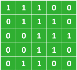
First of all, what does "convolution" even mean? In computer science and image processing, the convolution is a mathematical operation used to extract features from an image. (The formal mathematical definition is a little bit different.) The convolution is defined by an image kernel. The image kernel is nothing more than a small matrix. For instance, a 3x3 kernel matrix is very common. Remember that we can think of an image as a array of numbers. For simplicity let's just look at greyscale images at first.
For instance, say this is our image. (Where we have 1 being black and 0 being white).
And this is our 3x3 kernel.

The kernel is applied to the image by sliding it over the image and for each position computing the element wise multiplication of the two matrices and then summing up the result.
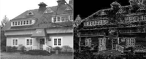
A different kernel will obviously produce a different output. The kernel can be specially selected to perform certain operations on the output image, such as edge detection, sharpening or blurring. Below is an example of an edge detection kernel of \( \begin{bmatrix} -1 & -1 & -1 \\ -1 & 8 & -1 \\ -1 & -1 & -1 \end{bmatrix} \) applied to an image.
We can also use multiple kernels to extract multiple different features from an image. A demonstration of this is shown below. First, the red kernel is slid over the input image to extract the first feature map (which is just the result of the convolution), and next, a different kernel colored in green does the same to produce a different feature map.
A large part of the reason why the convolution operator is such a powerful feature detector is that it is space invariant. Since the kernel slides over the entire image, it does not matter where in the image a given "feature" may be; the kernel will detect it regardless. Furthermore, the kernel is applied uniformly (the values of the kernel do not change as it is slid over the image), so it will detect a feature the same in one part of an image as another.
Still confused about the convolution operator? Check out this incredible demo for an interactive way to explore convolution.
The core idea of the CNN is to learn the values of these filters through backpropagation, and to stack multiple layers of feature detectors (kernels) on top of each other for abstracted levels of feature detection.
Sparse Connections
Another advantage of using convolutions instead of flattening our vectors and feeding them into a regular neural network is that they can still get pretty good results without needing so many neuron connections.
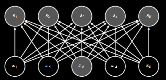
In traditional neural networks, each neuron is connected to every neuron in the next level. If a given layer has \( m \) inputs and \( n \) outputs, the runtime of the matrix multiplication needed to compute the layer output is \( O( m * n) \). The connections of a fully connected layer are shown below.
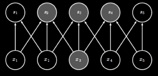
However, say we limit the number of connections each node has to \( k \). The runtime of such an approach is now \( O(k * n) \), where \( k \) is orders of magnitude smaller than \( m \)
Convolutional Layer Design
The convolution layer is at the core of a CNN. Recall that a standard neural network layer takes a vector as input. A CNN takes a volume as input. We will see how this concept makes sense soon. The neurons of a convolution layer are likewise arranged as volumes. The weights of a convolution layer can be viewed as a set of filters (from the convolution operator).
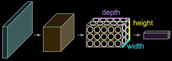
There are two primary concepts that make the convolution layer possible. The first is local connections. Just as explained above, this makes it so that each neuron, which can be thought of as one filter after being placed in a specific location on the image, is only connected to nearby points on the image. In terms of convolutional layers, this means that as the filter is slid across the image, only certain patches of the input layer are connected to the filter at any given point in time. The size of this patch is called the receptive field, or the filter size, and is the same as the dimension of the kernel (e.g. 3x3, 5x5). However, the connectivity is always full along the depth axis, so for a colored image, each filter is applied across every RGB channel. So in summary, connections are local in width and height, while full in the depth dimension.
Say an input volume is 32x32x3, meaning it is a 32x32 RGB image (3 color channels). We say that this image has 3 depth slices, each of which has an area of 32x32 (where each depth slice corresponds to one of the color channels). If we choose a filter size of 5x5 in this situation, then each neuron in the convolution layer would be connected to \( 5*5*3 = 75 \) weights (not including the bias). Note that this 5x5 filter size had to be connected to the full extent of the depth dimension (i.e. color channels).
As we will see shortly, it makes sense to call the incoming weights of the neuron a filter.
So how many neurons in the convolution layer are needed, and what local patches are these neurons connected to? The hyper parameters of depth, stride and zero padding address all of this.
Depth is the the number of neurons looking at the same local region of input. This will control the depth of the output volume. Since each neuron can be viewed as a filter, this controls the number of filters in the layer, and determines the number of image features that we want our layer to be able to detect. Each of these filters will be trained to detect some unique feature on the same input region.
Stride specifies how to slide a filter over the input region. Stride is essentially the step size that we will use when sliding our filter over the image. For instance, if the stride is 2, the filter will move 2 pixels at a time, skipping the pixel in the middle. This can be viewed as a form of image downsampling, because higher strides will produce smaller output volumes.
Zero padding is simply padding the input image with 0's around the edges. A zero padding of 3 would add 3 rings of zero-valued pixels around the borders of the image. Since applying convolutions to an image can shrink the image around the borders (as explained in the Computerphile video), zero padding gives us a way to control the output volume without having to choose between smaller spatial extent or smaller kernels.
The output volume size is dependent on the input volume size \( W \), the filter size \( F \) of the neurons, the stride \( S \), and the amount of zero padding \( P \). The output volume height and width is given by the following formula. $$ \frac{W - F + 2P}{S} + 1 $$ For a 32x32 input and a 5x5 filter with a stride of 1 and zero padding of 0, we would get a 28x28 output. Of course, fractional pixel values do not make sense, so there are some combinations of \(W, F, P\) and \( S \) that do not work.
The depth of the output layer is controlled by the depth of the neurons. We can notate this parameter as \( K \).
As another example, now say that the filter size is 11, the stride is 4, depth is 96 and that we use no zero padding. Say the input volume has a size of 227x227x3. Using the above formula, we can deduce that the output of the first layer will have dimensions of 55x55x96. All 96 neurons along a depth column are connected to the same input region of dimension 11x11x3.
Parameter Sharing
In the above example, we would have a total of 55*55*96 = 290,400 neurons in just the first layer, with each neuron having 11*11*3 weights (and 1 bias). Together, this adds up to over 100 million parameters. This number can be reduced through parameter sharing. Parameter sharing makes the assumption that it is useful for a filter to calculate the same features across the entire region of a depth slice. We can take advantage of this assumption by making all the neurons in single depth slice share the same weights and biases. So now, instead of 55*55*96 neurons, there are only 96 unique neurons. And as before, each of those 96 neurons is connected to a 11*11*3 volume giving \( 96*11*11*3 = 34,848 \) parameters (not including biases).
Now, if all the neurons in a single depth slice are using the same weights, then computing the forward pass of a convolution layer is the same as doing the convolution of the neuron's weights and the input volume. This is why we refer to the sets of weights for each neuron to be a filter or a kernel.
The same rules that applied to regular neural networks also apply to CNNs. The same concepts of backpropagation still apply, and the network is still composed of numerous layers and a loss function. Let's take a closer look at what these filters are computing. Below is an image of 96 filters in the first layer of a convolutional neural network used in image detection.
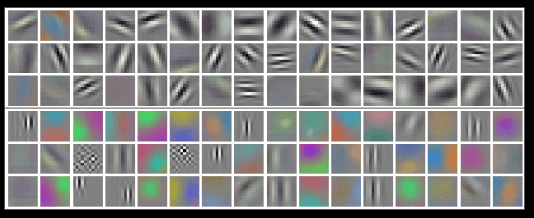
Remember that by the assumption of parameter sharing, we are assuming that if a filter learns that detecting a horizontal edge at some location in the image, is important it will be important at all locations of the image. This is a fair assumption to make, since images are typically invariant to translation. (i.e. if a picture of a cat has a cat in the top left hand corner, it is still a picture of a cat if the cat is moved to the opposite corner).
A fantastic resource for really getting a solid grasp on how the whole process work is the convolution demo made for the Stanford 231n course. A quick note before checking out the demo: this demo is for when there are two filters of size 3, a stride of 2, and a zero-padding of 1. Note that the filter weight matrices are both composed of 3 3x3 matrices because the input volume has a depth of 3. You may find it helpful to spend a good amount of time studying the demo and getting a good grasp on what is happening. Please find the demo here.
While the convolution layer is certianly the driving innovation behind CNNs there a few other layers that are usually incorporated into CNNs as well.
Pooling Layers
The role of pooling layers is to reduce the dimensionality of the input. Pooling layers are typically used right after convolution layers. Reducing the dimensionality of the input reduces the number of parameters we need to process the input, and by reducing complexity of the network, can help combat overfitting.
The pooling layer operates over every depth slice and does nothing to change the depth of the input. However, the output height and width are reduced by sampling from certain areas of the image, and then tossing the other areas.
The most common type of pooling is max pooling. Max pooling takes only the maximum pixel value from a region of pixels. So for instance, for a max pooling operation with filter size 2x2 and a stride of 2 would reduce a 8x8 image to a 2x2 image. Typically, the stride of the filter is just equal to the filter size. In the image below, each color of the image is a region that the pooling considers independently of the other regions.
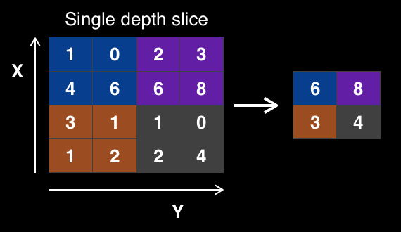
Max pooling actually makes the network a more powerful feature detector, as only the areas with maximum response to the convolution operator are kept. This preserves the most important features while throwing out the less important features.
And with that, we are one step closer to having all the building blocks to a convolutional neural network!
CNN Architecture
Fully Connected Layers
Before putting together a complete CNN, we first have to know that convolutional layers alone cannot make up a neural network that is capable of outputting a final prediction vector, which we need for classification and regression. (For example, this vector could represent the probabilities that an image shows a cat, dog, bird, etc.) Convolutional layers only output 3D volumes (or 2D areas), which are tensors, not vectors.
The basic architecture of a CNN is to stack successive layers of convolution and max pooling. However, after several convolution-max pooling pairs, the original image has been sufficiently processed to form a low dimensional, meaningful signal. Since we use convolutions to detect certain features in an input image, more positive values in this signal mean that the convolutional layers have successfully detected a certain abstract feature in the image (e.g. eyes, ears, a tail, etc.). (See the Computerphile videos above for some great visualizations of this process.)
At this point, it makes sense to make some sort of decision based on the signal produced by all of the convolution layers. The output of the convolution or max pooling layer is then flattened and passed through several fully connected layers. These fully connected layers are just the basic neural network connections presented in a previous tutorial on neural network basics. Two or three of these fully connected layers followed by an output layer is common.
This fully connected network at the end of the CNN is referred to as the decision network. This is because it takes the signal from the convolution layers, and makes a meaningful decision from it. We can think of these fully-connected layers as taking in the processed signal as "votes", and then deciding from these votes what the final outputted prediction should be. The output from these fully-connected layers then becomes the final output for our convolutional neural network.
Modern CNNs
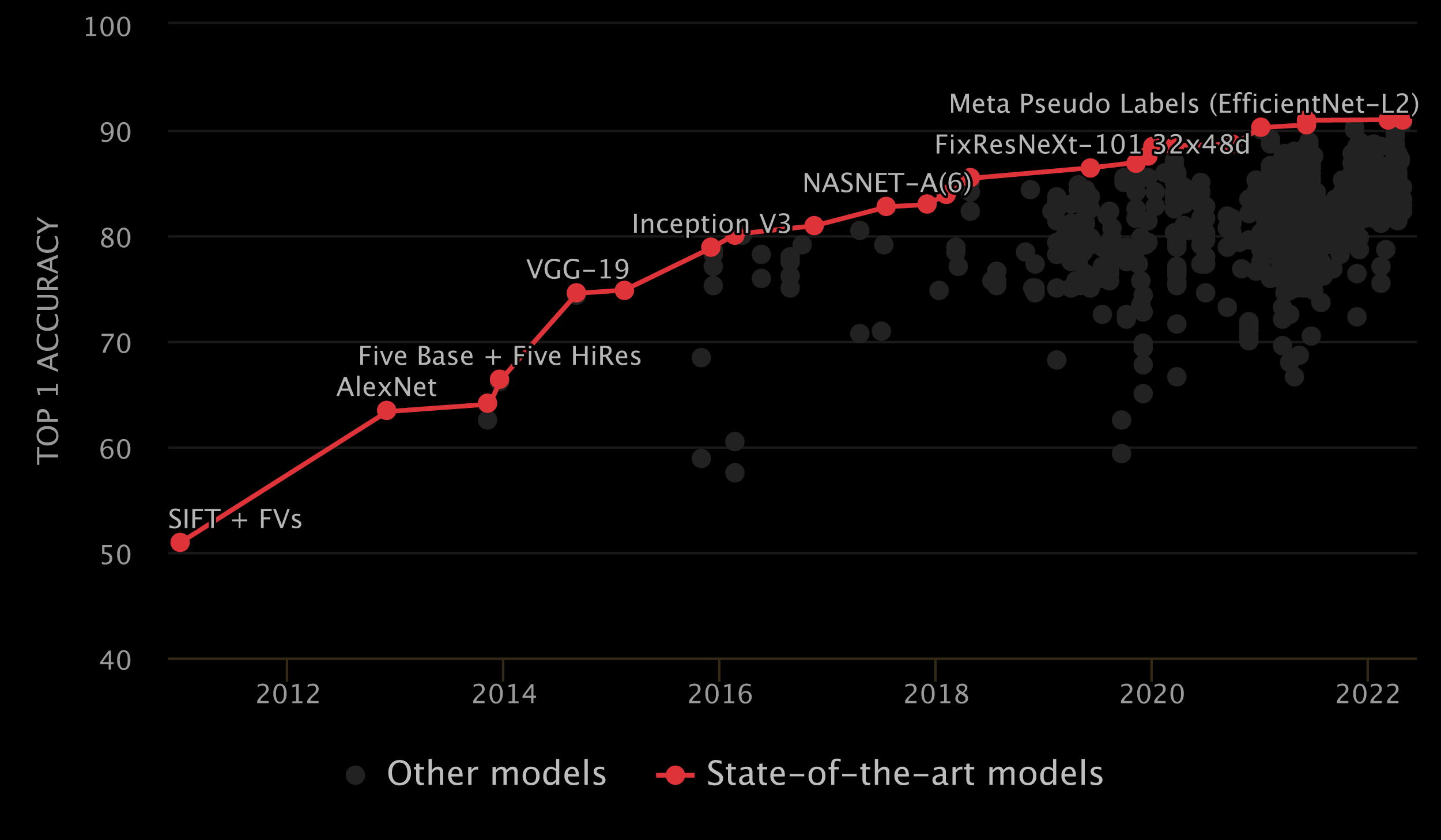
Now, let's take a look at actual CNN architectures. The development of CNNs have been a driving force behind the development of deep learning. As you will see, CNNs gradually got deeper and deeper during their development. Deeper CNNs are more powerful object detectors on high resolution images. This is only a small subset of the CNN architectures that are out there; newer, more powerful architectures are coming out every day.
-
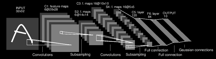
LeNet-5 (1998): This network is the original CNN, created
by Yann LeCun. It is often used as a
basic example for the MNIST dataset, which is comprised of 32x32x1 images of
handwritten digits (grey scale digits). The network architecture is in the following order:
- Convolutional layer composed of 6 5x5 filters. This reduces the input to 28x28x6.
- Downsampled by maxpooling that has a kernel size of 4 which gives an volume size of 14x14x6
- Convolution layer with 16 filters for 10x10x16.
- Max pooling layer reducing output to 5x5x16
- Flatten output
- Fully connected layer of 120 neurons
- Fully connected layer of 84 neurons
- Fully connected layer of 10 neurons
- Softmax function to determine class scores. (This was in the context of digit recognition and there are 10 digits)
- AlexNet (2012): This network has a very similar architecture to LeNet-5, so we will not go into the exact details. The first 5 layers are all convolution layers followed by a max pooling step, and the last 3 layers are fully connected layers.
-
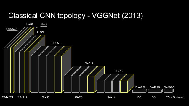
VGGNet (2013): This network was a step in the direction of very deep neural networks. It
showed that depth and layer-stacking were important to
improving the power of neural networks.
However, after VGGNet, network researchers struggled to come up with deep networks that could maintain the original features of the images. This led to the innovation of residual neural networks, which featured skip connections to allow networks to preserve original image features.
A visualization of the VGGNet architecture is shown below.
- ResNet (2015): This architecture takes advantage of residual or skip connections and allows for much deeper neural networks. Typically ResNets of 56 layers deep are employed.
-
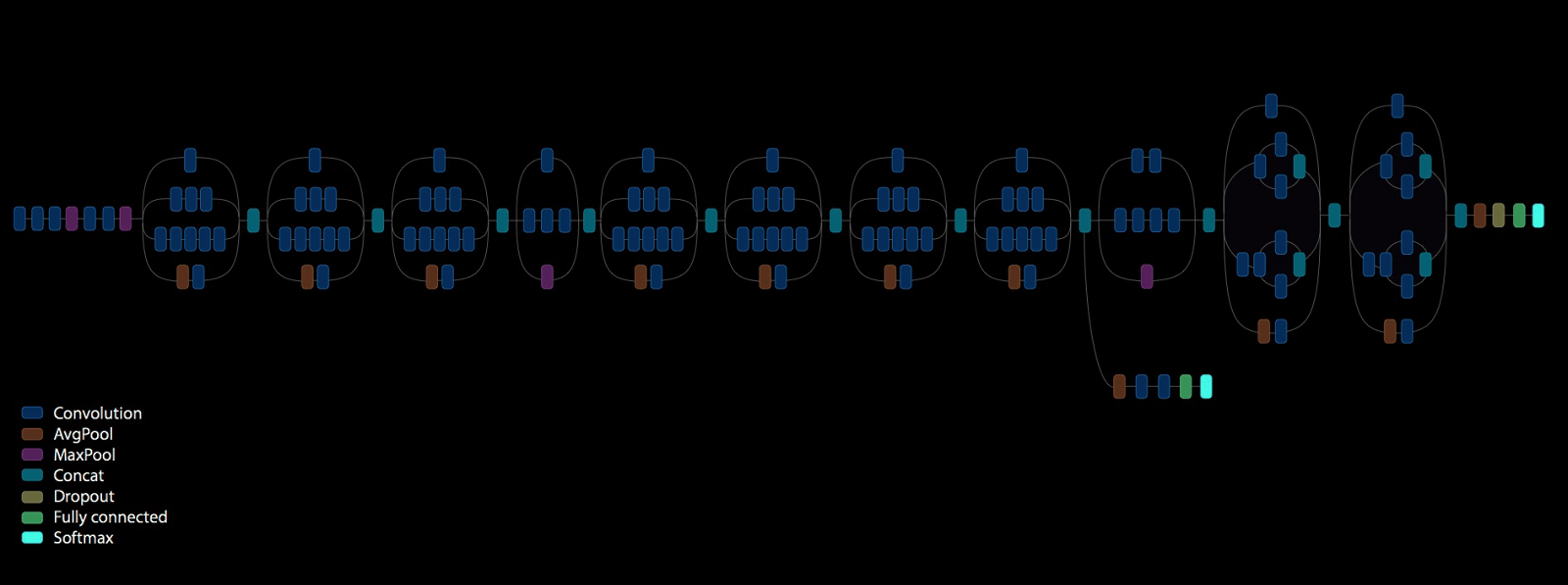
Inception v3 (2016): Google's Inception v3 network is a very deep neural
network that is currently (or as of writing this) state of the art in CNN
architectures. The network has 25 million trainable parameters and does 5
billion multiply-adds for a single forward pass through.
-
and more (++): Novel research is always coming out that improves on previous work and is able to break
through the current state of the art.
You might be wondering how people came up with such models. As of writing this, the experts in the field are largely also unsure as to why deep neural networks perform so well. As a result, the design process for these new networks typically consists of adding more layers and trying new things with the network until something works. This process has been referred to as Grad Student Descent (a joke on gradient descent that mocks grad students who iteratively guess network architectures without reason to desperately get a paper published).
Applications in Society
Now that we know what the sophisticated models are, we can get to where the real fun begins. Convolutional neural networks are much more than just an academic proof of concept: turns out, they can be used to help solve problems beyond just the realm of computer science — and in many instances, they already have. When organizations have lots of spatially-structured data that they want to better understand, machine learning is there to lead the way.
Below are some examples of how convolutional neural networks have been, and currently are being, applied in the real world. Our hope is that through continuing to use these cutting-edge technologies in positive ways, people will eventually come to see these technologies not as something to fear, but rather as a potential force for good. After going through this lesson, perhaps you, too, could think of a new way to use this exciting technology to help better the world around us.
How are CNNs being used for social good? (Just to name a few examples)
- Medicine: analyzing 3D lung scans to spot lung cancer (Data Science Bowl 2017)
- Environmentalism: detecting deforestation from satellite imagery (Kaggle Competition)
- Transportation: creating safer self-driving cars (NVIDIA: Paper, Blog)
- Wildlife Protection: training drones to patrol for poachers and animals from the sky (USC Teamcore)
Main Takeaways
- How convolutional filters scan images to look for specific spatial features
- Types of layers in ConvNets and their respective purposes: convolution (Conv), max pooling (MaxPool), rectified linear (ReLu), fully connected (FC)
- What happens to spatial data as it gets passed forward through a convolutional neural network (Hint: think “abstraction”)
- How Conv filters in later layers (i.e. farther from the input layer) may differ from Conv filters in earlier layers (i.e. closer to the input layer) after being trained (Hint: once again, think “abstraction”)
- When to use ConvNets as opposed to regular neural networks
- How ConvNets can and have been used in the real world