Background: Neural Machine Translation
In this article, we discuss the Transformer, a machine learning architecture largely born under the context of Neural Machine Translation (NMT). NMT was a problem that attempts to build a single, large model that reads an input text and outputs a translation: think Google Translate.
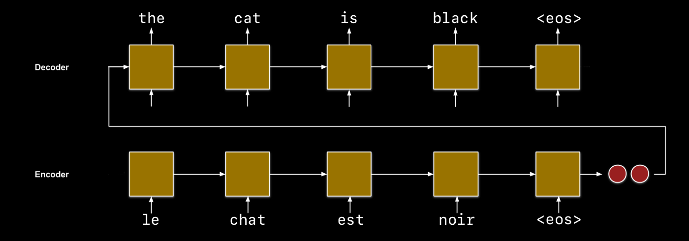
For a full understanding, we will introduce the history of architectures proposed to tackle NMT starting with a simple framework that leverages Recurrent Neural Networks (RNN) called sequence-to-sequence (seq2seq), proposed by [Sutskever et al. 2014].
The seq2seq approach uses an RNN (the encoder) to learn latent representations and an RNN (the decoder) to produce useful output.
For example, let’s say our challenge is to translate sentences from French to English. The encoder will read input word embeddings, from the French language, sequentially as they are listed in the sentence. In theory, the final hidden state produced by the encoder condenses the information described by the input sentence. Next, the decoder reads in the encoding and produces the translated English word embeddings.
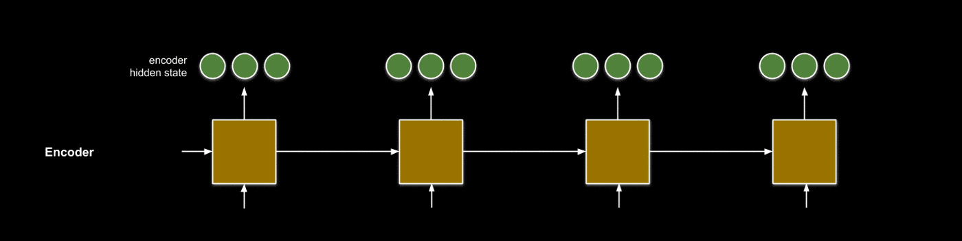
An issue with this seq2seq approach arises when the inputs and outputs become lengthy. As you might imagine, encoding a paragraph’s worth of information within a hidden state with a fixed length may not yield all the information originally contained within the sentence. Given an input sequence length \(N\), we want to be able to consider not only the final hidden state \(z_N\) but each hidden state \(z_1, ..., z_N\).
Attention, explained
You should be familiar with the concept of a weighted sum, which assigns a different importance weight \(w_i\) to each element \(z_i\) of a series before taking the sum of the series. The weighted sum is a technique to condense the amount of information in a vector to our liking.
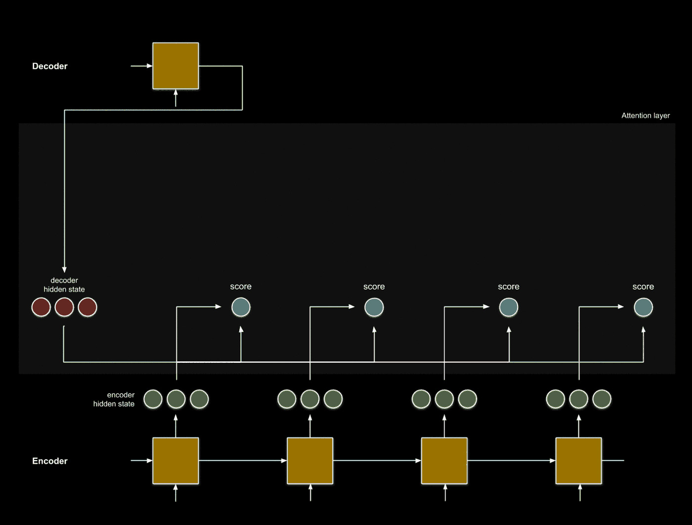
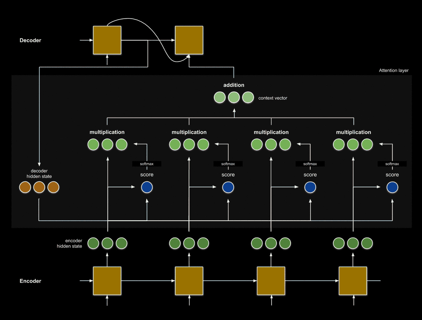
\[s = \sum_i w_i z_i\]A mechanism called attention leverages the weighted sum to condense the hidden states to information most relevant to a search key. In seq2seq, attention acts as an interface that provides the decoder with information about each hidden encoder state. We can use this information to complement decoder hidden states to produce translated outputs. This process is broken down into four steps.
1. Forward pass the input embeddings.
2. Using an attention score function, find a relationship.
The relationship we are trying to analyze is that between the decoder hidden state \(h_i\) and each encoder hidden state \(z_1, ..., z_N\). One common function to do this the dot product, which measures the similarity between two vectors.
This process enables us to examine which input words \(x_1, ... x_N\) are most related to the decoder word at index \(i\).
3. Take a weighted sum of the attention scores.
We want to condense the information relating to the decoder state \(h_i\) into a single vector, which we can accomplish by using the attention scores as weights. Note that instead of taking the element-wise sum of individual embeddings, we are taking the vector sum of all embeddings.
To take this sum fairly, we normalize the scores so that the sum of the scores is 1 using the softmax function.
The resulting vector is called the context vector, which describes the context surrounding decoder state \(h_i\).
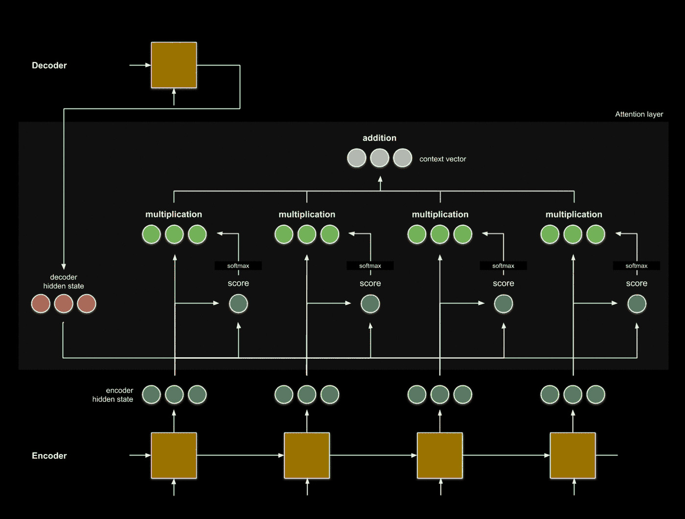
4. Leverage the context to inform translation.
We can use the context vector to inform our translation task. This step can be as simple as utilizing the context vector as additional input to our decoder.
Summary
And that’s it! We are now able to consider the context of each word in relation with other words to produce translated outputs, making translation of long sequences more robust to forgetting information.
There are many potential adaptations of this approach to alter performance: for example, we can tweak the encoder and decoder architectures to make the RNNs more complex, we can try different attention score functions, or we can use a different method of combining decoder hidden states and context vectors.
In our next section, we will discuss the memory and time limitations of seq2seq in favor of a more computationally efficient and powerful architecture, the transformer.
Transformers: Attention is All You Need
Three years after seq2seq, [Vaswani et al. 2017] proposed a novel architecture that refutes the need for RNNs for sequence transduction tasks, called the transformer. This architecture relies solely on attention to provide contextual information for sequence transduction. Similar to seq2seq, the transformer also relies on an encoder and decoder. The transformer encoder’s purpose is to provide context vectors from the input embeddings, and the decoder’s purpose is to predict the next element in the transduction sequence.
![]()
To understand the transformer, we first introduce self-attention, a self-supervised method to learn contextual information about a sequence.
Self-Attention: The Query, the Key, and the Value
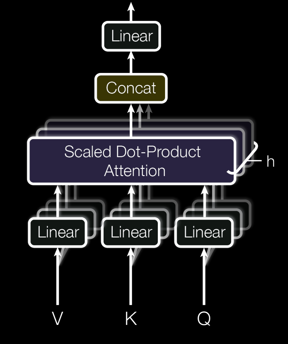
There are three uses for input embeddings in self-attention: (1) as a search token, the query; (2) as a retrieval token, the key; (3) the information value, the value. These three uses suggest an architecture that learns three different vectors for each input embedding. We can accomplish this by using weight matrices \(W_Q, W_K, W_V\) respectively (or identically, three fully-connected layers in parallel, as opposed to in series).
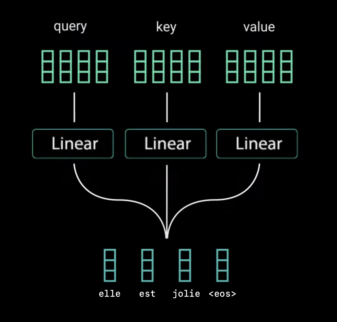
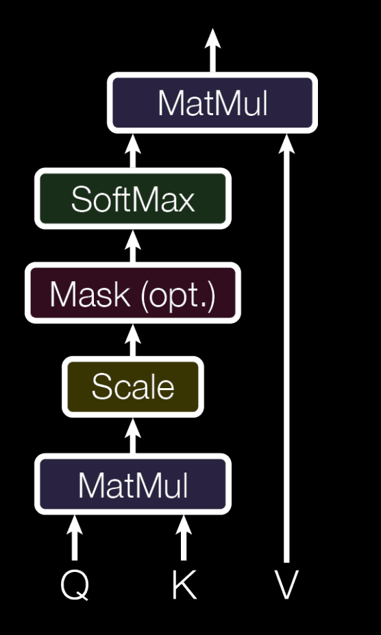
Next, we compute the attention score using a matrix multiplication between the queries \(W_QX\) and the keys \(W_KX\). These are also often denoted as \(Q\) and \(K\) respectively. This step is analogous to computing attention scores between the hidden decoder states and hidden encoder states in seq2seq, but note that we are only computing attention using the same input, hence why we call this self-attention.
Finally, we scale by dividing by \(\sqrt{d_k}\), the square root of the dimension for \(Q, K\), and we apply the softmax function to the attention scores so that they are properly normalized. We scale the output before applying the softmax function to reduce the effects of vanishing gradients. We can apply a matrix multiplication on the normalized attention score and the value \(V=W_VX\) to produce the context vector for each input embedding.
\[\text{Attention}(Q, K, V) = \text{softmax}(\frac{QK^T}{\sqrt{d_k}})V\]This is the premise of self-attention, which is illustrated in the figure below. You can ignore the masking layer for now, which we will discuss in detail in the decoder section.
Multi-Head Attention
One of the strengths of the transformer is its ability to produce different independent contexts using multiple weight matrices to produce \(Q, K, V\). This is called multi-head attention.
We can produce multi-head attention easily by having an extra three linear layers for each head. Since we can only have one context vector per input embedding, we will concatenate and apply a final linear layer to combine information from each attention head.
The Encoder
You now know the key elements of the transformer’s encoder.
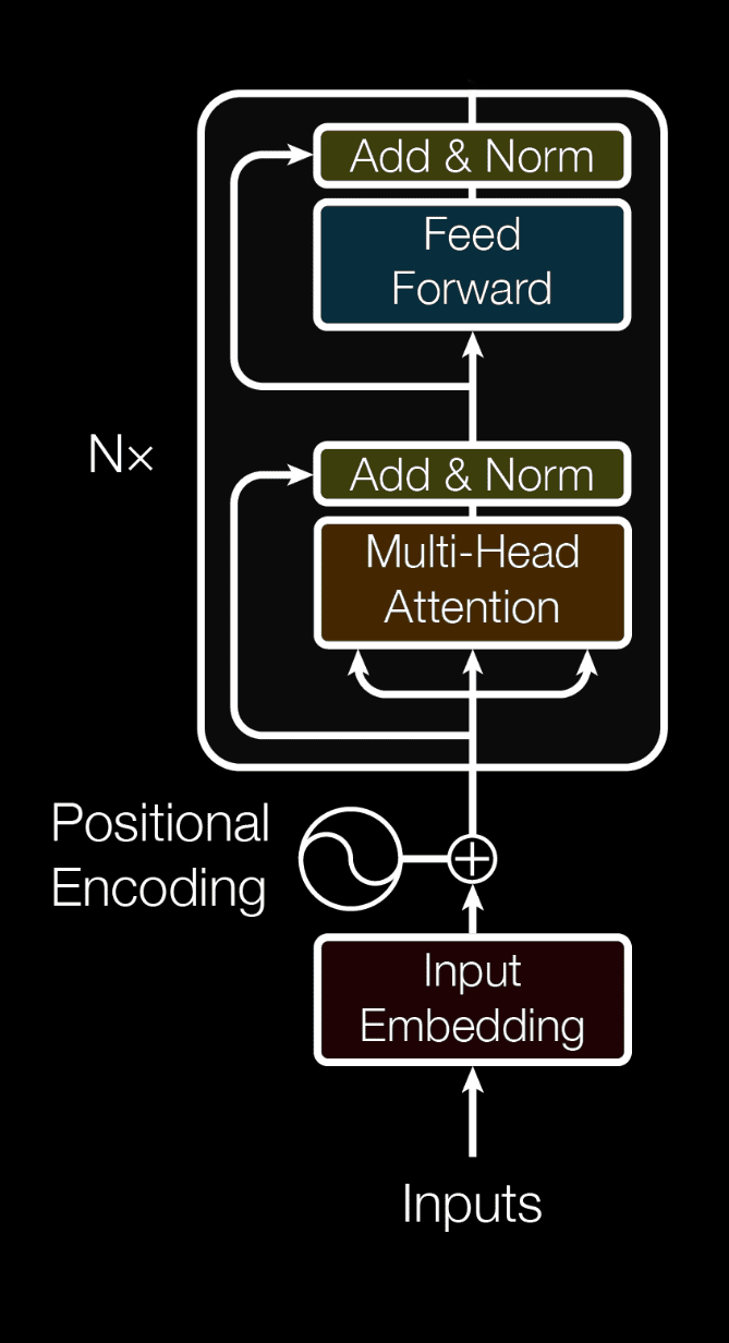
As opposed to seq2seq, the transformer computes each element of a sequence all at once, making the operation more computationally efficient. However, this lacks the positional information of each element in the sequence. We can provide the positional information by adding a positional encoding to the input embeddings. There are many choices for positional encoding functions, but it is not important to understand the details of this to understand the transformer. [Vaswani et al. 2017] uses a sinusoidal function to produce positional encodings:
\[PE_{(pos,2i)}=sin(pos/10000^{2i/d_{model}})\] \[PE_{(pos,2i+1)}=cos(pos/10000^{2i/d_{model}})\]In addition, the additional arrows that skip layers are known as residuals and help with vanishing gradients as well as providing original information about each embedding.
The \(N\times\) on the side indicates that the transformer encoder may be stacked in series many times, potentially improving the performance of the transformer.
And that’s it for the encoder! We have successfully produced context vectors from the sequential data using our transformer encoder’s multi-head attention blocks.
The Decoder
The decoder architecture is very similar to that of the encoders, but there are a few key differences. Instead of a regular multi-head attention block, we apply a masked multi-head attention block. The purpose of this masking is to prevent our attention block from seeing future elements in the sequence.
We make many passes over the decoder: each pass enables the decoder to predict one new word. For instance,
\[\begin{align} & \text{Encoder Input: Elle est jolie <eos>}\rightarrow \text{\{context\}}\\ \\ & \text{Decoder}\\ & \text{Step 0 Input: <bos> + \{context\}} \rightarrow \text{She}\\ & \text{Step 1 Input: <bos> She + \{context\}}\rightarrow \text{is}\\ & \text{Step 2 Input: <bos> She is + \{context\}}\rightarrow \text{pretty}\\ & \text{Step 3 Input: <bos> She is pretty + \{context\}}\rightarrow \text{<eos>}\\ \end{align}\]The architecture to produce this is the same as the encoder, except we mask future words in the multi-head attention block, insert an additional multi-head attention block that uses the encoder’s context vectors as \(Q, K\) and the decoder’s context vector as \(V\), and we add a linear classifier at the end.
![]()
Summary
The transformer is a very powerful architecture that is able to leverage attention in sequence transduction tasks. One such example is OpenAI’s GPT-3. There is some evidence GPT-3 can solve literary reasoning problems in standardized testing like the SAT. Play around with GPT-3 on this GPT-3 playground.