Introduction
In this section, we’ll take care of a few loose ends that we may have skimmed over in the previous lessons. These topics will become especially relevant for when you try to implement neural networks in your own projects.
Loss Functions
In our equations of backpropagation, we have used a generalized loss function \( J \). This cost function is what we aim to through stochastic gradient descent (SGD) and tells us how well the model is doing given the model parameters.
In earlier lessons, we saw the mean squared error used as a loss function. However, the mean squared error may not always be the best cost function to use. In fact, a more popular loss function is the cross entropy cost function. Before we get more into the cross-entropy cost function, let's look into the softmax classification function.
Softmax Classifier
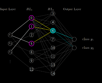
Let's say you are building a neural network to classify between two classes. Our neural network will look something like the following image. Notice that there are two outputs \( y_1 \) and \( y_2 \) representing class one and two respectively.
We are given a set of data points \( \textbf{X} \) and their corresponding labels \( \textbf{Y} \). How might we represent the labels? A given point is either class one or class two. The boundary is distinct. If you remember the linear classification boundary from earlier we said that any output greater than 0 was class one and any output less than 0 was class two. However, that does not really work here. A given data point \( \textbf{x}_i \) is simply class one or class two. We should not have data points be more class one than other data points.
We will use one hot encoding to provide labels for these points. If a data point has the label of class one simply assign it the label vector \( \textbf{y}_i = \begin{bmatrix} 1 \\ 0 \end{bmatrix} \) and for a data point of class two assign it the label vector \( \textbf{y}_i = \begin{bmatrix} 0 \\ 1 \end{bmatrix} \)
Say our network outputs the value \( \begin{bmatrix} c_1 \\ c_2 \end{bmatrix} \) where \(c_1, c_2 \) are just constants. We can say the network classified the input as class one if \( c_1 > c_2 \) or classified as class two if \( c_2 > c_1 \). Let's use the softmax function to interpret these results in a more probabilistic manner.
The softmax function is defined as the following $$ q(\textbf{c}) = \frac{e^{c_i}}{\sum_j e^{c_j}} $$ Where \( c_i \) is the scalar output of the \(ith\) element of the output vector. Think of the numerator as converting the output to an un-normalized probability. Think of the denominator as normalizing the probability. This means that for every output \( i \) the loss function will have an output between 0 and 1. Another convenient property of the softmax function is that the sum of all the output probabilties \( i \) will sum to \( 1 \), making this activation function more suitable to working with probability distributions.
Entropy
We need to take one more step before we can use the softmax function as a loss function. This requires some knowledge of what entropy is. Think about this example. Say you were having a meal at EVK, one of the USC dining halls. If your meal is bad, this event does not carry much new information, as the meals are almost guaranteed to be bad at EVK. However, if the meal is good, this event carries a lot of information, since it is out of the ordinary. You would not tell anyone about the bad meal (since a bad meal is pretty much expected), but you would tell everyone about the good meal. Entropy deals with this measure of information. If we know an underlying distribution \( y \) to some system, we can define how much information is encoded in each event. We can write this mathematically as: $$ H(y) = \sum_i y_i \log \left( \frac{1}{y_i} \right) = - \sum_i y_i \log ( y_i ) $$
Cross Entropy
This definition assumes that we are operating under the correct underlying probability distribution. Let's say a new student at USC has no idea what the dining hall food is like and thinks EVK normally serves great food. This freshman has not been around long enough to know the true probability distribution of EVK food, and instead assumes the probability distribution \( y'_i \). Now, this freshman incorrectly thinks that bad meals are uncommon. If the freshman were to tell a sophomore (who knows the real distribution) that his meal at EVK was bad, this information would mean little to the sophomore because the sophomore already knows that EVK food is almost always bad. We can say that the cross entropy is the encoding of events in \( y \) using the wrong probability distribution \( y' \). This gives $$ H(y, y') = - \sum_i y_i \log y'_i $$
Now let's go back to our neural network classification problem. We know the true probability distribution for any sample should be just the one hot encoded label of the sample. We also know that our generated probability distribution is the softmax function. This gives the final form of our cross entropy loss. $$ L_i = -\log \left( \frac{e^{c_i}}{\sum_j e^{c_j}} \right) $$ Where \( y_i = 1 \) for the correct label and \( y' \) is the softmax function. This loss function is often called the categorical cross entropy loss function because it works with categorical data (i.e. data that can be classified into distinct classes).
And while we will not go over it here, know that this function has calculable derivatives as well. This allows it to be used just the same as the mean squared error loss function. However, the cross entropy loss function has many desirable properties that the mean squared error does not have when it comes to classification.
Let's say you are trying to predict the classes cat or dog. Your neural network has a softmax function on the output layer (as it should because this is a classification problem). Let's say for two inputs \( \textbf{x}_1,\textbf{x}_2 \) the network respectively outputs $$ \textbf{a}_1 = \begin{bmatrix} 0.55 \\ 0.45 \end{bmatrix}, \textbf{a}_2 = \begin{bmatrix} 0.44 \\ 0.56 \end{bmatrix} $$ where the corresponding labels are $$ \textbf{y}_1 = \begin{bmatrix} 1 \\ 0 \end{bmatrix}, \textbf{y}_2 = \begin{bmatrix} 0 \\ 1 \end{bmatrix} $$ As you can see, the network only barely classified each result as correct. But by only looking at the classification error, the accuracy would have been 100%.
Take a similar example where the output of the network is just slightly off. $$ \textbf{a}_1 = \begin{bmatrix} 0.51 \\ 0.49 \end{bmatrix}, \textbf{a}_2 = \begin{bmatrix} 0.41 \\ 0.59 \end{bmatrix}, \textbf{y}_1 = \begin{bmatrix} 0 \\ 1 \end{bmatrix}, \textbf{y}_2 = \begin{bmatrix} 1 \\ 0 \end{bmatrix} $$ Now in this case, we would have a 0% classification accuracy.
Let's see what our cross entropy function would have given us in each situation when averaged across the two samples. In the first situation: $$ -(\log(0.55) + \log(0.56)) / 2 = 0.59 $$ In the second situation: $$ -(\log(0.49) + \log(0.59)) / 2 = 0.62 $$ Clearly, this result makes a lot more sense for our situation than just having a cost value of \( 0 \) for a barely-correct classification.
Overall, the choice of the correct loss function is dependent on the problem, and is a decision you must make in designing your neural network. Always keep in mind the general equations for stochastic gradient descent will have the form: $$ \mathbf{W} (k) = \textbf{W}(k-1) - \alpha \nabla J(\textbf{x}_k, \textbf{W}(k-1)) $$ $$ \mathbf{b} (k) = \textbf{b}(k-1) - \alpha \nabla J(\textbf{x}_k, \textbf{b}(k-1)) $$ Where \( J \) is the loss function. Furthermore, the same form of backpropagation equations will still apply with backpropagating the error terms through the network.
Optimization: Mini-Batch Algorithm
First let's review our SGD algorithm shown below. Note that \( \theta \) is commonly used to refer to all the parameters of our network (including weights and biases). $$ \mathbf{\theta} (k) = \mathbf{\theta}(k-1) - \alpha \nabla J(\textbf{x}_k, \mathbf{\theta}(k-1)) $$ As this algorithm is stochastic gradient descent, it operates on one input example at a time. This is also referred to as online training. However, this is not an accurate representation of the gradient, as it is only over a single training input, and is not necessarily reflective of the gradient over the entire input space. A more accurate representation of the gradient could be given by the following. $$ \mathbf{\theta} (k) = \mathbf{\theta}(k-1) - \alpha \nabla J(\textbf{x}, \mathbf{\theta}(k-1)) $$ The gradient at each iteration is now being computed across the entire input space. This is referred to as batch gradient descent, which actually turns out to be a kind of confusing name in practice (as we'll see in a bit).
In practice, neither of these approaches are desirable. The first does not give a good enough of an approximation of the gradient -- the second is computationally infeasible, since for each iteration, the gradient of the cost function for the entire dataset has to be computed. Mini-batch methods are the solution to this problem.
In mini-batch training, a sample set of all the training examples are used to compute the cost gradient. The average of these gradients for each sample is then used. This approach offers a good trade off between speed and accuracy. The equation for this method is given below, where \( Q \) is the number of samples in the mini-batch and \( \alpha \) is the learning rate. $$ \mathbf{\theta} (k) = \mathbf{\theta}(k-1) - \frac{\alpha}{Q} \sum_{q=1}^{Q}\nabla J(\textbf{x}_q, \mathbf{\theta}(k-1)) $$ Remember that batch gradient descent is over the whole input space, while mini-batch is just over a smaller subset at a time.
Of course, it would make sense that the samples have to be randomly drawn from the input space, as sequential samples will likely have some correlation. The typical mini-batch sampling procedure is to randomly shuffle the input space, and then to sample sequentially from the scrambled inputs.
Optimization: Initializations
At this point, you may be wondering how the parameters of a neural network are typically initialized. So far, the learning procedure has been described, but the actual initial state of the network has not been discussed.
You may think that how a network is initialized does not necessarily matter. After all, the network should eventually converge to the correct parameters right? Unfortunately, this is not the case with neural networks; as it turns out, the initialization of the parameters matters greatly. Initializing to small random weights typically works. But typically, the standard for weight initialization is the normalized initialization method.
In the normalized initialization method, weights are randomly drawn from the following uniform distribution: $$ \textbf{W} \sim U \left( -\frac{6}{\sqrt{m+n}}, \frac{6}{m+n} \right) $$ Where \( m \) is the number of inputs into the layer and \( n \) is the number of outputs from the layer.
As for the biases, typically just assigning them to a value of 0 works.
Challenges in Optimization
In mathematical optimization, we optimize (i.e. find the minimum/maximum of) some function \( f \). In machine learning, we can think of training a neural network as a specific type of optimization (gradient descent) applied to a specific cost function.
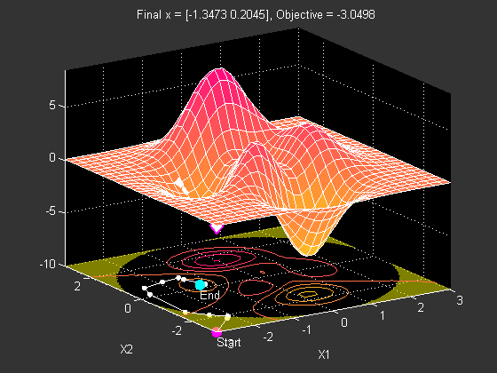
As you may have expected, there are some concerns that can arise in this training phase: for example, local minima. Any deep neural network is guaranteed to have a very large number of local minima. Take a look at the below surface. This surface has two minima: one local, and one global. If you look at the contour map below, you can see that the algorithm converges to the local minimum instead of the global minimum.
Should we take measures to stop our neural network from converging at a local (rather than a global) minimum? Local minima would be a concern if the cost function evaluated at the local minima was far greater than the cost function evaluated at the global minima. It turns out that in practice, this difference is often negligible. Most of the time, simply finding any minima is sufficient in the case of deep neural networks.
Some other potential problem points are saddle points, plateaus, and valleys. In practice, neural networks can often escape valleys or saddle points. However, they can still pose a serious threat to neural networks, since they can have cost values much greater than at the global minimum. Even more dangerous to the training process are flat regions on the cost surface. Small initial weights are chosen in part to avoid these flat regions.
In general, more flat areas are problematic for the rate of convergence. It takes a lot of iterations for the gradient descent algorithm to get over flatter regions. One's first thought may be to increase the learning rate of the algorithm, but too high of a learning rate will result in divergence at steeper areas of the performance surface. When this algorithm with a high learning rate goes across something like a valley, it will oscillate out of control and diverge. An example of this is shown below.
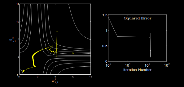
At this point, it should be clear that several modifications to backpropagation need to be made to allow solve this oscillation problem and to fix the learning rate issue.
Momentum
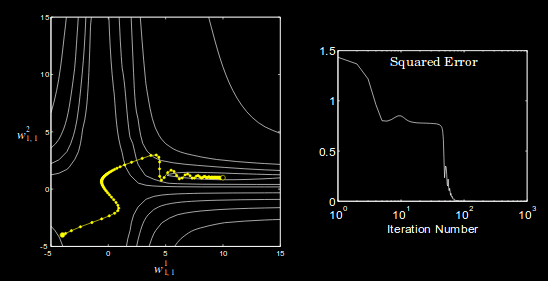
For this concept, it is useful to think of the progress of the algorithm as a point traveling over the cost surface. Momentum in neural networks is very much like momentum in physics. And since our 'particle' traveling over the cost surface has unit mass, momentum is just the velocity of our motion. The equation of backprop with momentum is given by the following. $$ \textbf{v}(k) = \lambda \textbf{v}(k-1) - \alpha \nabla J(\textbf{x}, \mathbf{\theta}(k-1)) $$ $$ \mathbf{\theta} (k) = \mathbf{\theta}(k-1) + \textbf{v}(k) $$ The effect of applying this can be seen in the image below. Momentum dampens the oscillations and tends to make the trajectory continue in the same direction. Values of \( \lambda \) closer to 1 give the trajectory more momentum. Keep in mind that \( \lambda \) itself does not actually represent the magnitude of the particle's momentum; instead, it is more like a force of friction for the particle's trajectory. Typical values for \( \lambda \) are 0.5, 0.9, 0.95 and 0.99.
Nesterov momentum is an improvement on the standard momentum algorithm. With Nesterov momentum, the gradient of the cost function is considered after the momentum has been applied to the network parameters at that iteration. So now we have: $$ \textbf{v}(k) = \lambda \textbf{v}(k-1) - \alpha \nabla J(\textbf{x}, \mathbf{\theta}(k-1) + \lambda \textbf{v}(k-1)) $$ $$ \mathbf{\theta} (k) = \mathbf{\theta}(k-1) + \textbf{v}(k) $$ In general, Nesterov momentum outperforms standard momentum.
Adaptive Learning Rates
One of the most difficult hyper-parameters to adjust in neural networks is the learning rate. Take a look at the image below to see the effect of learning different learning rates on the minimization of the loss function.
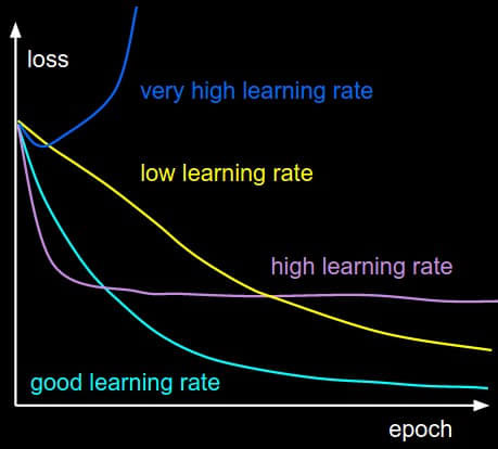
As from above, we know that the trajectory of the algorithm over flat sections of the cost surface can be very slow. It would be nice if the algorithm could have a fast learning rate over these sections, but a slower learning rate over steeper and more sensitive sections. Furthermore, the direction of the trajectory is more sensitive in some directions as opposed to others. The following algorithms will address all of these issues with adaptive learning rates.
AdaGrad
The Adaptive Gradient algorithm (AdaGrad) adjusts the learning rate of each network parameter according to the history of the gradient with respect to that network parameter. This is an inverse relationship, so if a given network parameter has had large gradients (i.e. steep slopes) in the recent past, the learning rate will scale down significantly.
Whereas before there was just one global learning rate, there is now a per parameter learning rate. We set the vector \( \textbf{r} \) to be the accumulation of the parameter's past gradients, squared. We initialize this term to zero. $$ \textbf{r} = 0 $$ Next we compute the gradient as usual $$ \textbf{g} = \frac{1}{Q} \sum_{q=1}^{Q}\nabla J(\textbf{x}_q, \mathbf{\theta}(k-1)) $$ And then accumulate this gradient in \( r \) to represent the history of the gradient. $$ \textbf{r} = \textbf{r} + \textbf{g}^2 $$ And finally, we compute the parameter update $$ \mathbf{\theta} (k) = \mathbf{\theta}(k-1) - \frac{\alpha}{\delta + \sqrt{\textbf{r}}} \odot g $$ Where \( \alpha \) is the global learning rate, and \( \delta \) is an extremely small constant ( \( 10^{-7} \) ). Notice that an element wise vector multiplication is being performed (by the \( \odot \) operator). Remember that each element of the gradient represents the partial derivative of the function with respect to a given parameter. The element wise multiplication will then scale the gradient with respect to a given parameter appropriately. The global learning rate is usually not difficult to choose, and normally works as just 0.01.
However, a problem with this algorithm is that it considers the whole sum of the squared gradient since the beginning of training. In practice, This results in the learning rate decreasing too much too early.
RMSProp
RMSProp is regarded as the go-to optimization algorithm for deep neural networks. It is similar to AdaGrad, but includes a decay over the accumulation of the past gradient-squared, so the algorithm "forgets" gradients far in the past.
As normal, compute the gradient. $$ \textbf{g} = \frac{1}{Q} \sum_{q=1}^{Q}\nabla J(\textbf{x}_q, \mathbf{\theta}(k-1)) $$ Now, this is where the algorithm changes with the introduction of the decay term \( \rho \), which is set somewhere between 0 and 1. $$ \textbf{r} = \rho \textbf{r} + (1 - \rho) \textbf{g}^2 $$ And the parameter update is the same. $$ \mathbf{\theta} (k) = \mathbf{\theta}(k-1) - \frac{\alpha}{\delta + \sqrt{\textbf{r}}} \odot g $$
Second Order Algorithms
Second order algorithms make use of the second derivative to "jump" to the critical points of the cost function. Further discussion of these algorithms is outside the scope of this tutorial. However, these algorithms do not work very well in practice. First of all, it is computationally infeasible to compute the second order derivatives. Second of all, for a complex performance surface with many critical points, it is very likely the second order method would go in the completely wrong direction. Overall, gradient descent first order methods have been shown to perform better, so I would not worry about knowing what second order algorithms are all about. But know that they exist and are an active area of research.
Regularization (Continued)
Recall from our previously that regularization is a technique that we can use to reduce overfitting by producing more robust models that are more capable of making general predictions in the real world. In this section, we’ll discuss a variety of specific methods that we can use to address this problem of overfitting.
Parameter regularization aims to reduce overfitting by penalizing for overly complex models. We can do this by adding an extra term to our cost function that penalizes large weights (which usually indicate overfitting), which helps result in smoother model predictions. This type of regularization defines the parameter norm penalty as the following. $$ \Omega(\theta) = \frac{1}{2} \lVert \textbf{w} \rVert_2^2 $$ and the total objective function: $$ \hat{J}(\theta, \textbf{X}, \textbf{y}) = J(\theta, \textbf{X}, \textbf{y}) + \frac{\alpha}{2} \textbf{w}^T \textbf{w} $$ Evidently, this regularization will penalize larger weights. In theory, this should help prevent the model from overfitting. It is common to employ \( L^2 \) regularization when the number of observations is less than the number of features. Similar to \( L^2 \) regularization is \( L^1 \), which you can probably expect is just \( \Omega(\theta) = \frac{1}{2} \lVert \textbf{w} \rVert_1 \). In almost all cases, \( L^2 \) regularization outperforms \( L^1 \) regularization.
Early Stopping
When we are working with a dataset, we split that dataset up into testing and training datasets. The training dataset is used to adjust the weights of the network. The test dataset is used to check the accuracy of the model on data that has never been seen before.
However, the training dataset can be divided again into the training data and a small subset of data called the validation set. The validation set is used during training to ensure that the model is not overfitting. (You can think of the validation set as lying somewhere between the training set, which is used at every step of the training process, and the test set, which is only used at the very end of the training process to evaluate the model's generalizability.) This validation data is not ever used to train the model. The validation accuracy refers to the model's accuracy over the validation set. The goal is to minimize the validation accuracy through tuning hyperparameters of the network. The network is only evaluated on the test dataset with the fully tuned model.
Take a look at the below graph showing validation loss versus training loss. It should be clear that at a certain point, the model overfits on the training data and begins to suffer in validation accuracy despite this not being reflected in the training accuracy.
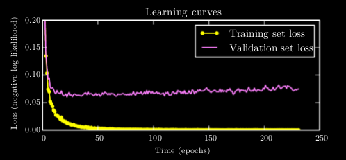
The solution to this is to simply stop training once the validation set loss has not improved for some time. Just like \( L^1 \) and \( L^2 \) regularization, this is a method of decreasing overfitting on the training dataset.
Ensemble Methods
Bagging (short for bootstrap aggregation, a term in statistics) is the technique of making a model generalize better by combining multiple weaker learners into a stronger learner. Using this technique, several models are trained separately and their results are averaged for the final result. This ideal of one model being composed of several independent models is called an ensemble method. Ensemble methods are a great way to fine tune your model to make it generalize better on test data. Ensemble methods apply to more than just neural networks, and can be used on any machine learning technique. Almost all machine learning competitions are won using ensemble methods. Often times, these ensembles can be comprised of dozens and dozens of learners.
The idea is that if each model is trained independently of each other, they will have their own errors on the test set. However, when the results of the ensemble learners are averaged the error should approach zero.
Using bagging, we can even train a multiple models on the same dataset but be sure that the models were trained independently. With bagging, \( k \) different datasets of the same size are constructed from the original dataset for \( k \) learners. Each dataset is constructed by sampling from the original dataset with some probability with replacement. So there will be duplicate and missing values in the constructed dataset.
Furthermore, differences in model initialization and hyperparameter tuning can make ensembles of neural networks particularly favorable.
Dropout
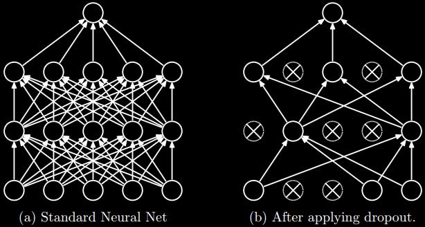
Dropout is a very useful form of regularization when used on deep neural networks. At a high level, dropout can be thought of randomly removing neurons from some layer of the network with a probability \( p \). Removing certain neurons helps prevent the network from overfitting.
In reality, dropout is a form of ensemble learning. Dropout trains an ensemble of networks where various neurons have been removed and then averages the results, just as before. Below is an image that may help visualize what dropout does to a network.
Dropout can be applied to input units and hidden units. The hyperparameter of dropout at a given layer is the probability with which a neuron is dropped. Furthermore, another major benefit of dropout is that the computational cost of using it is relatively low. Finding the correct probability will require parameter tuning because a probability too low and dropout will have no effect, while too high and the network will be unable to learn anything.
Overall, dropout makes more robust models and is a standard technique employed in deep neural networks.
The Unstable Gradient Problem
As a final section, let's go over a problem in optimization that plagued the deep learning community for decades.
As we've seen, deeper neural networks can be a lot more powerful than their shallow counterparts. Deeper layers of neurons add more layers of abstraction for the network to work with. Deep neural networks are vital to visual recognition problems. Modern deep neural networks built for visual recognition are hundreds of layers deep.
However, you may think that you can take what you have learned so far build a very deep neural network and expect it to work. However, to your surprise you may see that adding more layers at a certain point does not seem to help and even reduces the accuracy. Why is this the case?
The answer is in unstable gradients. This problem plagued deep learning up until 2012, and its relatively recent solutions are responsible for much of the deep learning boom. The cause of the unstable gradient problem can be formulated as different layers in the neural network having vastly different learning rates. And this problem only gets worse with the more layers that are added. The vanishing gradient problem occurs when earlier layers learn slower than later layers. The exploding gradient problem is the opposite. Both of these issues deal with how the errors are backpropagated through the network.
Let's recall the equation for backpropagating the error terms through the network. $$ \delta^{m} = f'(\textbf{z}^{m}) \left( \textbf{W}^{m + 1} \right)^{T} \delta^{m+1} $$ Now let's say the network has 5 layers. Let's compute the various error terms recursively through the network. $$ \delta^5 = \frac{\partial J}{\partial \textbf{z}^5} $$ $$ \delta^4 = f'(\textbf{z}^4)(\textbf{W}^{5})^T \frac{\partial J}{\partial \textbf{z}^5} $$ $$ \delta^3 = f'(\textbf{z}^3)(\textbf{W}^{4})^T f'(\textbf{z}^4)(\textbf{W}^{5})^T \frac{\partial J}{\partial \textbf{z}^5} $$ $$ \delta^2 = f'(\textbf{z}^2)(\textbf{W}^{3})^T f'(\textbf{z}^3)(\textbf{W}^{4})^T f'(\textbf{z}^4)(\textbf{W}^{5})^T \frac{\partial J}{\partial \textbf{z}^5} $$ $$ \delta^1 = f'(\textbf{z}^1)(\textbf{W}^{2})^T f'(\textbf{z}^2)(\textbf{W}^{3})^T f'(\textbf{z}^3)(\textbf{W}^{4})^T f'(\textbf{z}^4)(\textbf{W}^{5})^T \frac{\partial J}{\partial \textbf{n}^5} $$ The term for \( \delta^1 \) is massive, and this is only for a five layer deep network. Imagine what it would be for a 100 layer deep network! The important take away is that all of the terms are being multiplied together in a giant chain.
For a while, the sigmoid function was believed to be a powerful activation function. The sigmoid function and its derivative are shown below.
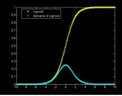
Say we were using the sigmoid function for our five layer neural network. That would mean that \( f' \) is the function shown in red. What is the maximum value of that function? It's around 0.25. What types of values are we starting with for the weights? Small random values. The key here is that the values start small. The cause of the vanishing gradient problem should now start becoming clear. Because of the chain rule, we are recursively multiplying by terms less far less than one, causing the error terms to shrink and shrink going backwards in the network.
With this many multiplication terms, it would be something of a magical balancing act to manage all the terms so that the overall expression does not explode or shrink significantly.
How do we fix this problem? The answer is actually pretty simple. Just use the ReLU activation function instead of the sigmoid activation function. The ReLU function and its derivative are shown below.
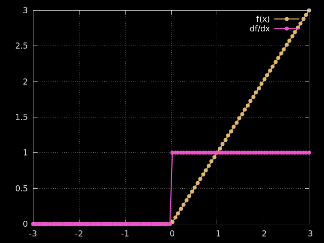
As you can see, its derivative is either 0 or 1, which alleviates the unstable gradient problem. This function is also much easier to compute.
References
- http://neuralnetworksanddeeplearning.com
- http://hagan.okstate.edu/NNDesign.pdf
- https://www.amazon.com/Deep-Learning-Adaptive-Computation-Machine/dp/0262035618
- http://cs231n.github.io/
- https://jamesmccaffrey.wordpress.com/2013/11/05/why-you-should-use-cross-entropy-error-instead-of-classification-error-or-mean-squared-error-for-neural-network-classifier-training/