Introduction
In previous lessons we have seen different types of neural networks, all of which solve regression or classification problems. We started with plain vanilla neural networks, which take a vector as input and pass it through some hidden layers to produce the output. We then added to this design to form new types of networks. For example, convolutional neural networks are well-suited for spatially organized data, making them a good choice for image classification. Recurrent neural networks are well-suited for sequential or temporal data, and thus excel at natural language processing. Here we introduce another type of network called a Generative Adversarial Network (GAN). These were first conceived in a paper published in 2014 by Ian Goodfellow et al. Unlike the others, this one does not solve regression or classification problems. It belongs to a special class of models called generative models, meaning its purpose is to create something, not classify something. GANs can learn to mimic almost any distribution of data we give it. There are many other types of generative models - variational autoencoders and boltzmann machines to name a few - however GANs come with their own set of advantages that lead many to regard them as the state of the art in generative modeling.
Specifically, GANs generate new data by taking a game theory approach. A GAN takes two neural networks and pits them together in a game, where each network tries to outperform the other. But much like in real life, when you play a game against a worthy adversary, you learn from them. Both networks learn from each other, and the end result is two high-performing neural networks, one of which is capable of generating brand new data.
One example of what a GAN might be able to do is generate images of dogs. We have already succeeded in classifying images as dogs (or cats) in our convolutional neural network workshop. However, image generation is a different task. More concretely, a traditional neural network takes a high-dimensional input and transforms it down to a low-dimensional output representing the prediction. We want to go in the opposite direction: take a low-dimensional input (such as 1 for dog or 0 for cat) and output a higher-dimensional image of a dog or cat. There are many correct answers to this task, and GANs consider all of them. Here is another way to think about it: classifiers try to predict p(y|x), while GANs predict p(x|y). In other words, GANs figure out how likely it is for a feature to show up in an image with label y.
Generator vs. Discriminator
GANs are comprised of two major components, a generator and a discriminator. These are both neural networks, and we put them together to give the overall functionality of the GAN. The discriminator is nothing new, it is a traditional neural network that classifies its input by outputting a number. It is often implemented as a convolutional neural network, but it can be other types of neural networks too. The generator is different: it can be thought of as the “reverse” of a traditional neural network. It takes a low-dimensional input, often just a random distribution of noise, and produces a high-dimensional output, such as an image of what it believes to be a dog. To get a high-level sense of how these two pieces fit together, look at the image below:
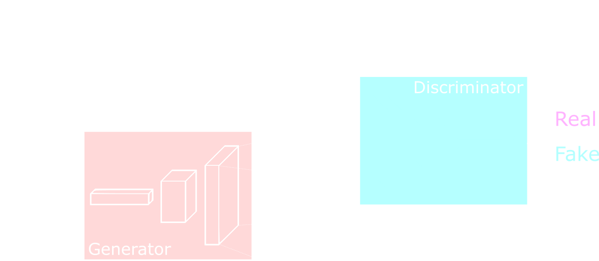
The discriminator is fed both real images from the dataset, as well as fake ones made by the generator. Its goal is to determine which ones are fake and which ones are real, encoding its answer as a 1 or 0. The two networks are connected by piping the output of the generator to the input of the discriminator, and then training is conducted on the entire construction. The training process uses backpropagation and gradient descent just like before, with a few slight changes discussed below.
Here is one analogy commonly used to help grasp this concept. Think of the discriminator as the police and the generator as a criminal who makes fake ID’s. At first, the criminal is not very smart, and the ID’s he produces are clearly fake. But after being caught by the police a few times, the criminal learns how to make the ID’s more realistic. Eventually he is able to fool the police. But then, the police adapt more sophisticated methods to catch fake ID’s, and the criminal must find a way to improve his ID’s even more. It is an ongoing battle between two adversaries: the police and the criminal, each getting better as the other improves.
Mathematically, here is the game that is being played:
\[\min_{\theta_{g}}\max_{\theta_{d}}\big[\mathop{\mathbb{E}_{x\sim p_{data}}}\log(D_{\theta_{d}}(x)) + \mathop{\mathbb{E}_{z\sim p(z)}}\log(1 - D_{\theta_{d}}(G_{\theta_{g}}(z)))\big]\]Where:
\(D\) is the output of the discriminator.
\(G\) is the output of the generator.
\(x\) is a real training sample.
\(z\) is a random noise distribution.
\(\theta\) is the set of parameters to be adjusted
The discriminator tries to maximize the expression in parentheses, while the generator tries to minimize it. Both networks do this by adjusting their parameters. Take a moment to look at this expression and convince yourself it does represent the game being played. Don’t worry too much about the \(\mathop{\mathbb{E}}\) symbol, you can just ignore it here - it means “on expectation.” The first term \(\log(D(x))\) represents the discriminator’s output when given real data, and the second term \(\log(1 - D(G(z)))\) represents one minus the discriminator’s output when given fake data. Think about what happens when the discriminator predicts close to 1 or 0; plug these numbers into the expression to see why the discriminator wants to maximize and the generator wants to minimize.
Generator
The generator takes as input a vector of random numbers, often called a latent sample. These random numbers are processed by the neural network to output a higher-dimensional piece of data, such as an image. In the case of image generation, you can think of the generator as a reverse convolutional neural network. ooking at the expression above, the parameters of the generator are adjusted to minimize the following function:
\[\min_{\theta_{g}}\big[\mathop{\mathbb{E}_{z\sim p(z)}}\log(1 - D_{\theta_{d}}(G_{\theta_{g}}(z)))\big]\]Note this is just the second term in the above expression, since the first term is out of the generator’s control (there is no \(\theta_{g}\)). This serves as the cost function for the generator, which we try to minimize using gradient descent. But in practice, it turns out this is not an effective way to train the generator. The reason is the gradient is very small in the early stages of training, so the parameters barely get adjusted and the generator learns very slowly. The gradient only gets respectably big towards the end of training. To alleviate this, we optimize this function instead:
\[\max_{\theta_{g}}\big[\mathop{\mathbb{E}_{z\sim p(z)}}\log(D_{\theta_{d}}(G_{\theta_{g}}(z)))\big]\]That is, rather than try to minimize the chance the discriminator is right, we maximize the chance the discriminator is wrong. Also notice how we are finding the maximum, not the minimum, of this function. This means we need to perform the opposite of gradient descent, sometimes called “gradient ascent.” Gradient ascent simply finds the parameters that correspond to the maximum of a function, rather than the minimum.
Once the parameters have been adjusted via gradient ascent, the generator should be able to create realistic samples of data that strongly resemble the training data.
Discriminator
The discriminator is the other half of the GAN. It takes in high-dimensional input, such as an image, and classifies it as real or fake. The discriminator works in exactly the same way as a standard neural network. But the key point to remember is that any given input will either be a real image from the training set or a fake image from the generator. Just like the generator, we adjust the parameters of the discriminator to maximize the following function:
\[\max_{\theta_{d}}\big[\mathop{\mathbb{E}_{x\sim p_{data}}}\log(D_{\theta_{d}}(x)) + \mathop{\mathbb{E}_{z\sim p(z)}}\log(1 - D_{\theta_{d}}(G_{\theta_{g}}(z)))\big]\]This is exactly the same as the expression representing the game, but without the \(\min_{\theta_{g}}\). Once training is completed, we actually throw out the discriminator. The generator is what we care about, the discriminator is simply a tool we use to train the generator.
Training
The generator and discriminator start off very unintelligent, and must improve by playing the game against each other. Take a look at this high-level pseudocode that explicitly steps through how a GAN is trained. Carefully walk through each step and try to understand what is happening, the notation is the same as above.
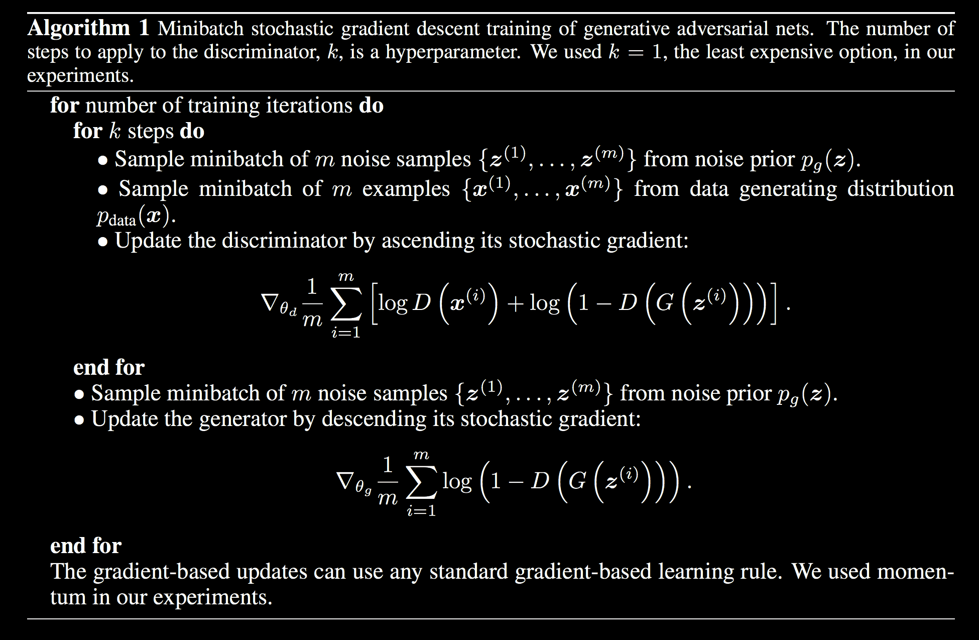
Note how we first train the discriminator a little bit, then switch to training the generator, then back to the discriminator, and so on until training is complete. In the second for loop we must choose a value for \(k\) which determines how many times we train the discriminator before switching to the generator. There are differing opinions on this; at the NIPS conference Ian Goodfellow said he finds \(k=1\) sufficient. Others argue for choosing a higher \(k\) so the generator and discriminator are not trained in a one-to-one fashion. The takeaway here is we can reasonably simplify this pseudocode by choosing \(k=1\), effectively removing the second for loop.
Additionally, while the generator is being trained, it is important to freeze the weights of the discriminator, and vice versa. Since both neural networks have different cost functions, we don’t want the training of one to interfere with the training of the other.
It is also important to adjust the learning rates of the generator and discriminator so they learn at about the same speed. If one learns much faster than the other, then we run into the vanishing gradient issue. Namely, the gradients will get very small for the network that is learning relatively slowly. Ongoing research has revealed other cost functions that can be used to avoid the vanishing gradient problem, however they are a more advanced topic.
Applications
Now let’s look at some pictures! In this section we see what GANs can do, and give some explanation as to what is going on in each research example.
Here is the first one: using GANs with some simple vector addition and subtraction, we can generate images based on combinations of other images. Take a look at this example, where a woman with sunglasses is generated without needing a training set containing of women with sunglasses.
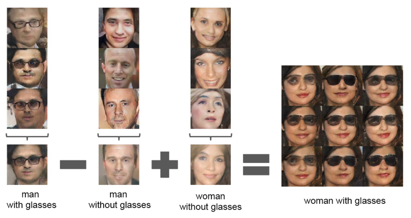
This example comes from a paper by Alec Radford and Luke Metz, and provides a great opportunity to talk more about latent space. First, imagine all image vectors represent a point in a high-dimensional space. This is often referred to as the latent space, and it turns out images that are generally similar have points in the latent space relatively close to each other. There are continuous paths through this space, which can be traversed by changing the values of the image vector components. This means it is possible to perform image addition and subtraction to construct new images. In other words, let’s say I’m given the latent vectors of the face of a man \(M\), the face of a man with sunglasses \(G\), and the face of a woman \(W\). Using vector addition and subtraction, the following expression would evaluate to an image vector of a woman wearing sunglasses: \(G-M+W\).
Let’s apply this to GANs by doing the same thing, using the example above. First use the generator to create a bunch of pictures of men with glasses, and average all of the input vectors \(z\) used to generate these images (note this random noise vector is still “high-dimensional,” although not as high as an image). Do the same for pictures of men without glasses, and women without glasses. Call these averaged vectors \(G'\), \(M'\) and \(W'\) respectively. Perform the same vector operation \(G'-M'+W'\) to get a new input vector that, when passed through the generator, will produce a woman wearing sunglasses. This works because all we are doing is moving through the latent space.
Another implication of this is we can generate images of dogs, for example, but also specify what its fur color, size, perspective angle, and any other feature should be. When generating an image of a dog there are many correct answers, but this manipulation of vectors throught the latent space allows us to be more specific.
Let’s take a look at the next study, which makes modifications to the GAN architecture to create what is referred to as a CycleGAN (see this paper).
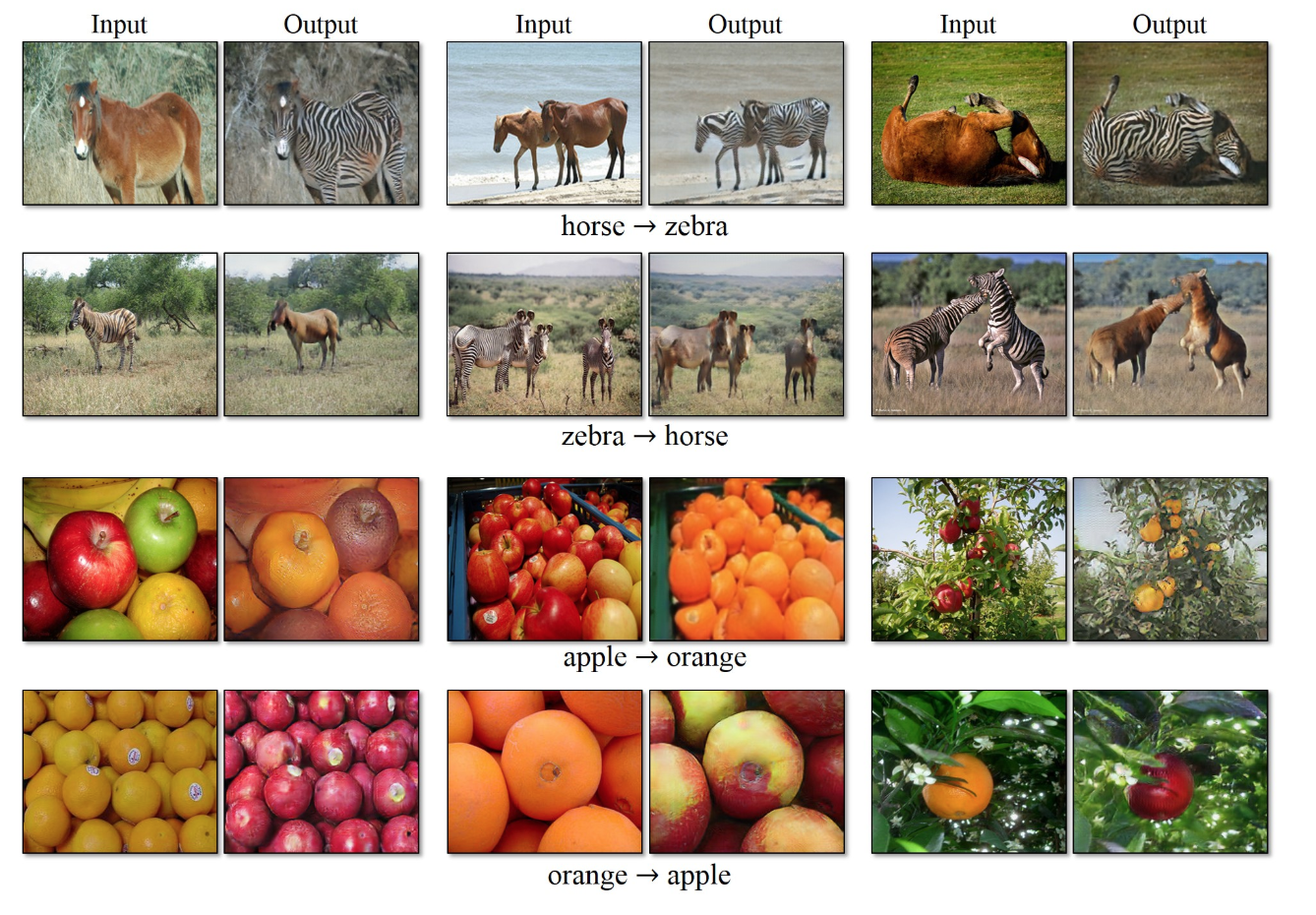
In this example, we can change the style of images through a process called domain transformation. Let’s use the first set of pictures of turning horses into zebras to explain. The horse belongs to a source domain we will call \(D_{a}\) and we wish to transfer it to the second domain \(D_{b}\) to make it look like a zebra. By putting two GANs together (for a total of 2 generators and 2 discriminators) we can move the images back and forth between these domains. Take a look at this architecture:
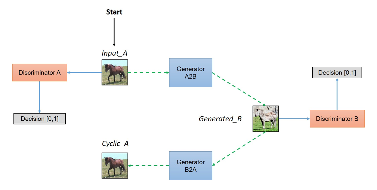
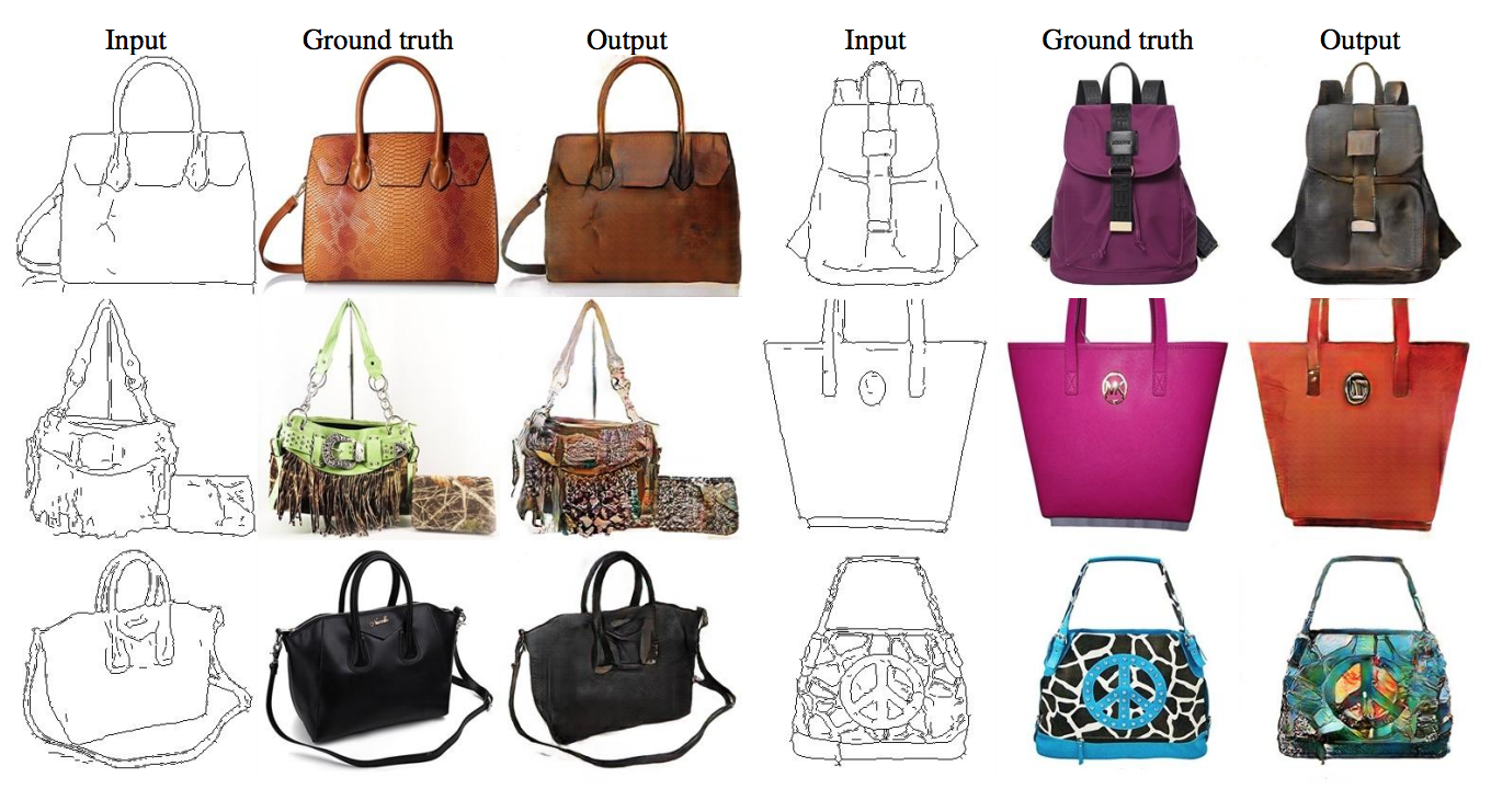
In this architecture, the adversary of Discriminator A is Generator B2A, while the adversary of Discriminator B is Generator A2B. If the image that is outputted by Generator B2A is extremely similar to the original image, then the CycleGAN has found a good mapping between the two domains. This means we don’t need to define the mapping ourselves - another key advantage to CycleGANs. A similar generative model called Pix2Pix requires explicitly providing this mapping to, for example, fill in sketches. As you can see here, each sketch must come from a “ground truth” that needs to be defined.
Here is yet another application of GANs, where text can be converted to images. Here is the paper on this.
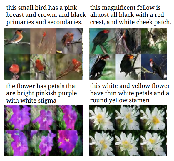
As you can see, there is much research on GANs and it is ongoing. They allow us to model nearly any distribution of data, even if we don’t directly have that data. People have sold artwork generated by GANs for hundreds of thousands of dollars - they really are exceptional at what they do.
Resources
- https://deeplearning4j.org/generative-adversarial-network
- https://www.analyticsvidhya.com/blog/2017/06/introductory-generative-adversarial-networks-gans/
- http://blog.aylien.com/introduction-generative-adversarial-networks-code-tensorflow/
References
- https://hackernoon.com/generative-adversarial-networks-a-deep-learning-architecture-4253b6d12347
- https://danieltakeshi.github.io/2017/03/05/understanding-generative-adversarial-networks/
- https://www.youtube.com/watch?v=Sw9r8CL98N0
- http://caisplusplus.usc.edu/curriculum
- http://papers.nips.cc/paper/5423-generative-adversarial-nets.pdf
- https://skymind.ai/wiki/generative-adversarial-network-gan
- https://arxiv.org/abs/1511.06434
- https://hardikbansal.github.io/CycleGANBlog/
- https://arxiv.org/abs/1703.10593
- https://arxiv.org/abs/1611.07004
- https://arxiv.org/pdf/1605.05396.pdf
- https://www.youtube.com/watch?v=5WoItGTWV54